Lab 3: Survival of the Fitter
Introduction
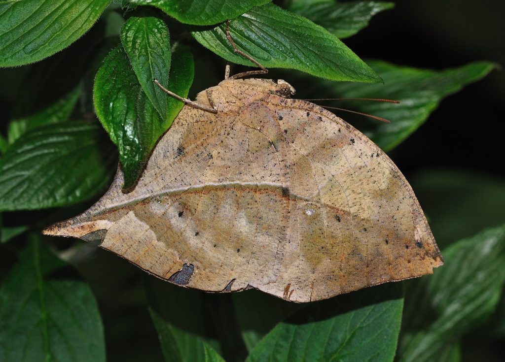
How does the saguaro survive in the harsh temperatures and extreme dryness of the desert? How is it that barnacles have developed the ability to endure pounding waves and daily exposure to the drying sun and wind of the intertidal zone? How did ducks come to have webbed feet? We commonly say that each of these species is adapted to its special set of conditions. But how did these species (and others) come to acquire traits that enable their living in particular environments?
The process of adaptation is explained by the theory of evolution developed independently, but simultaneously, by Charles Darwin and Alfred Wallace. According to the theory, shifts in phenotypic frequencies occur via natural selection, a process in which members of a population most suited for a particular set of environmental conditions will reproduce more successfully and pass on more of their genes than less suited members. Various factors of environmental resistance such as drought, predators, parasites, and even environmental pollutants are selective agents to the underlying genotypic shifts.
In this lab you are to investigate how natural selection works as you explore one example of how environmental pressures (selection pressure from predators) can drive changes in a population (of a prey species) over time – the predator-prey relationship.
Lab Objectives
In this lab, you will:
- Describe what is meant by the following terms: adaptation, natural selection, survival of the fitter, predator–prey interactions, coevolution.
- Work collaboratively to collect and analyze data and make graphs to visually represent the data.
- Apply your observations and data to discuss what is meant by natural selection and show how this may lead to change or evolution of populations.
- Explain how predator–prey interactions may cause an adaptive change in the prey population.
- Explain how predator–prey interactions may cause an adaptive change in the predator population.
- Explore how humans influence evolution and shape species and ecosystems.
Lab Directions
- Work in groups of 4.
- Count out 50 of each kind of bean (i.e., 50 garbanzo, 50 lentil, and 50 pinto) and scatter them widely on the mat provided. The beans represent the individuals of a prey population (a total of 150—the carrying capacity of the habitat). The different beans represent genetic variation among members of the population of a single species, Beanus beanus.
- The predator species is Flatwarus flatwarus and the knife, fork, and spoon represent genetic variations in the predator population. For the first simulation, three students will use a fork as the predator variant and paper cup to capture the prey (the beans).
- The fourth student is to act as a timekeeper.
- At the signal from the timekeeper, the “predators” are to proceed to catch the “prey.” They must pick prey off the mat (one at a time) using their forks and transfer the prey to their cup. Setting the cup on its side on the mat and pushing beans into it is not acceptable.
- Stop hunting at the end of 45 seconds. Time should be such that about one-half of the total number of beans are picked up in the allotted time (i.e., about 75), but if your group is significantly outside this range, adjust the hunting time accordingly and start over. If your group captured more than 75 prey (beans) reduce your hunting time such that you capture only about 75 prey (beans). On the other hand, if your group captured less than 75 prey (beans) increase your hunting time such that you capture about 75 prey (beans).
- When you have successfully accomplished the hunt (i.e., captured about 75 prey), it is the end of the first generation. Count the surviving prey by each bean variant. Each prey variant reproduces by adding the same number of each kind of bean that survives. For example, if 15 garbanzo, 14 pinto, and 49 lentils survived (remained on the mat at the end of the hunting time), add 15 garbanzo offspring, 14 pinto offspring, and 49 lentil offspring. Record the survivorship and reproduction for each prey variant in Table 3.1 on the Lab Response.
- Calculate the total population of each prey variant at the start of the next generation by adding the number of survivors to the number born. For the example in step 7 above, the total number of garbanzo beans will be 30 (15 survivors + 15 offspring), the total number of pinto beans will be 28 (14 survivors + 14 offspring), and the total number of lentils will be 98 (49 survivors + 49 offspring). These beans (prey) are then scattered widely on the mat for the second generation. (Reminder: At the start of each generation, there should be a total prey population of approximately 150, the carrying capacity for the habitat).
- Repeat steps 5-8 for 4 more generations. At the end of each generation, record the survivorship and reproduction for each prey variant in Table 3.1 on the Lab Response.
- Calculate the percent of the total population represented by each variant (i.e, bean type) in each generation and record under % of variant in Table 3.1. This has been calculated for the first generation (GEN 1).
- Carry out a second simulation to learn more about how natural selection operates. Use essentially the same setup but change the predator variant to knives. Observe the outcome in terms of differential survival and reproduction of prey. Record results on Table 3.2 on the Lab Response.
- Generate and upload two graphs of your data to the Lab Response. You can use the graphs provided or generate your own.
- From Table 3.1 graph the percentage of bean variants through the 6 generations for the fork simulation. Plot as a line graph showing the percent of the total population represented by each variant (i.e, bean type) over the 6 generations. Hence, there will be 3 plot lines on this graph, one line for each bean variant. Label each plot line and/or provide a legend. Also label the axes of the graph (if you generate your own graph). In addition, provide a brief interpretation of the graph.
- From Table 3.2 graph the percentage of bean variants through the 6 generations for the knife simulation. Plot as a line graph showing the percent of the total population represented by each variant (i.e, bean type) over the 6 generations. Hence, there will be 3 plot lines on this graph, one line for each bean variant. Label each plot line and/or provide a legend. Also label the axes of the graph (if you generate your own graph). In addition, provide a brief interpretation of the graph.
- Answer the questions on the Lab Response form.
Lab 3 Response: Survival of the Fitter
Download this Lab Response Form as a Microsoft Word document.
Data Tables
Table 3.1. Fill in data for each of the six generations of simulation 1.
Predator Variant: FORK
| GEN 1 | % of variant | Survivors | Reproduction | GEN 2 | % of variant | Survivors | Reproduction | |
|---|---|---|---|---|---|---|---|---|
| Garbanzo | 50 | 33.3% | ||||||
| Pinto | 50 | 33.3% | ||||||
| Lentil | 50 | 33.3% | ||||||
| TOTALS | 150 | 100% | 100% |
| GEN 3 | % of variant | Survivors | Reproduction | GEN 4 | % of variant | Survivors | Reproduction | |
|---|---|---|---|---|---|---|---|---|
| Garbanzo | ||||||||
| Pinto | ||||||||
| Lentil | ||||||||
| TOTALS | 100% | 100% |
| GEN 5 | % of variant | Survivors | Reproduction | GEN 6 | % of variant | |
|---|---|---|---|---|---|---|
| Garbanzo | ||||||
| Pinto | ||||||
| Lentil | ||||||
| TOTALS | 100% | 100% |
Predator Variant: KNIFE
| GEN 1 | % of variant | Survivors | Reproduction | GEN 2 | % of variant | Survivors | Reproduction | |
|---|---|---|---|---|---|---|---|---|
| Garbanzo | 50 | 33.3% | ||||||
| Pinto | 50 | 33.3% | ||||||
| Lentil | 50 | 33.3% | ||||||
| TOTALS | 150 | 100% | 100% |
| GEN 3 | % of variant | Survivors | Reproduction | GEN 4 | % of variant | Survivors | Reproduction | |
|---|---|---|---|---|---|---|---|---|
| Garbanzo | ||||||||
| Pinto | ||||||||
| Lentil | ||||||||
| TOTALS | 100% | 100% |
| GEN 5 | % of variant | Survivors | Reproduction | GEN 6 | % of variant | |
|---|---|---|---|---|---|---|
| Garbanzo | ||||||
| Pinto | ||||||
| Lentil | ||||||
| TOTALS | 100% | 100% |
For Figure 3.2, plot the data from Table 3.1.

Brief interpretation of Figure 3.2:
For Figure 3.3, plot the data from Table 3.2.
Brief interpretation of Figure 3.3:
Questions
- Respond to this question based on the predator–prey simulation using the FORK predator:
The Beanus (prey) population started with an equal number of individuals of each variant (garbanzo, lentil, and pinto). How did this change over the course of the experiment?
-
- Which variant(s) became more common in the total population? Explain why.
- Which variant(s) became less common in the total population or were eliminated? Explain why.
- Did any variant remain about the same in the total population? Explain why.
- Respond to this question based on the predator-prey simulation using the KNIFE predator:
The Beanus (prey) population started with an equal number of individuals of each variant (garbanzo, lentil, and pinto). How did this change over the course of the experiment?
-
- Which variant(s) became more common in the total population? Explain why.
- Which variant(s) became less common in the total population or were eliminated? Explain why.
- Did any variant remain about the same in the total population? Explain why.
- What is meant by “survival of the fitter” and why is it more appropriate to say “survival of the fitter” rather than “survival of the fittest”? Explain how this concept is demonstrated in this lab.
- How do the results of your lab simulation(s) of predator–prey evolution apply to natural predator and prey populations?
To answer this question:
-
- Explain how predator and prey populations adapt in response to each other (i.e., how the predator–prey interaction acts as the selection agent). Provide an example from natural predator and prey populations as part of your discussion.
- What is this particular evolutionary pattern called?
- Aside from biotic factors such as predator–prey interactions, abiotic factors also operate as selection agents on species. Identify two abiotic factors and provide examples from natural populations to illustrate how these factors have operated as agents of natural selection.
- Humans, as a biotic component of the ecosphere, have acted in many ways to directly or indirectly function as a selection agent for other species. Describe two specific examples of how human activities have operated as agents of selection on plant and animal species.
