3. Linear motion
Summary
Path and displacement
The concepts of path and displacement enable us to analyze how far an object moves as it travels. Path describes the total length of the motion of an object as it moves from one point to another, measured along its trajectory. It is a scalar quantity. The symbol that we use could be the lowercase letter d, the lowercase letter x, or the lowercase letter y. We typically use the letter d when discussing the concept of distance. We use the letter x when discussing a horizontal motion. We use the letter y when discussing a vertical motion. Either way, the units we use for path are meters (m).
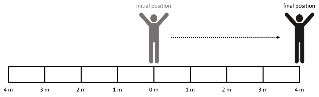
To demonstrate the concept of path, as depicted in Figure 3.1, a person starts at a position of 0 m (known as the origin). They walk at a mostly constant pace until they reach a position 4 m to the right of the origin. The person’s path describes the distance that they walked, which is equal to 4 m.
Displacement describes the straight-line distance from one point to another. It is a vector quantity, so it must include direction. The symbol that we use could be  ,
,  , or
, or  . The units of displacement are meters (m).
The uppercase Greek letter Delta ( ) means “change in.” Any physical quantity that can change has a final value and an initial value. A quantity starts at its initial value, and after a change is applied, ends up at the final value:

This equation can be rearranged by subtracting the initial value from both sides of the equation to allow us to solve for the change:

Therefore, every time an expression contains the symbol , it can be solved by subtracting the initial value of a quantity from the final value of that same quantity. Because is used in the symbols of displacement, it indicates that displacement is equal to an overall change in position between two points (a start and an end) and is equal to the final position minus the initial position.
Consider Figure 3.1 again. After starting at a position of 0 m and moving 4 m to the right of the origin, the person then moves to a position 2 meters to the left of the origin. This is shown in Figure 3.2.
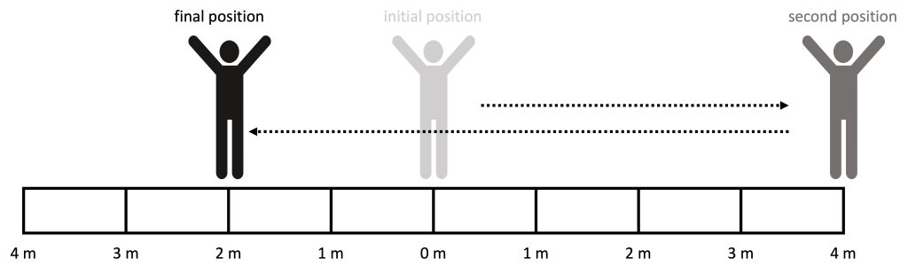
The path of the person after moving between these locations is the total distance that the person walked. From the origin to 4 m the person walked 4 m. From 4 m to the right of the origin to 2 m to the left of the origin, the person walked an additional 6 m. In this example, the total path is 10 m.
Displacement, on the other hand, only considers the change in position from the initial to final locations. The initial position is 0 m. The final position is -2 m (negative because it is to the left of the origin).

If, after all of this walking around, the person were to return to the origin, the total path would be 12 m (the first 4 m walking to the right, 6 m walking to the left, and then 2 m walking back to the origin). The total displacement would be zero. This is because the initial and final locations are the same.
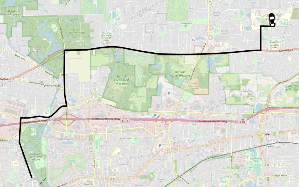
To further demonstrate the concepts of path and displacement, consider driving in a car from Naperville, Illinois, to the College of DuPage (COD). When driving a car, it isn’t always possible to go in a direct straight line. Instead, somebody driving a car has to follow the roads. This route describes the path of the car, and is shown in Figure 3.3.
The displacement between Naperville and the college only considers the straight-line distance between the starting and ending locations. Regardless of the path that’s taken to move between the two points, the displacement remains the same. It is always equal to the vector pointing from the starting point to the finishing point. This displacement vector is depicted in Figure 3.4. The displacement vector points to the northeast.
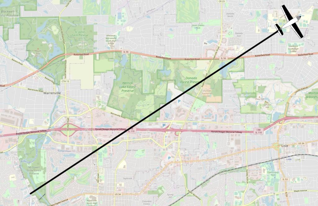
When driving in a car, you can determine your path by taking a look at your odometer. Unless you are able to drive in a completely straight line, it’s slightly more difficult to calculate the displacement as you drive from one place to another. However, if you know the coordinates of the starting and ending location, you can draw a straight line between two points. By splitting the straight line into horizontal and vertical components, you can use the Pythagorean theorem to calculate the displacement. The direction of the displacement can be determined by using a compass.
Speed and velocity
The concepts of speed and velocity enable us to analyze how fast (or slowly) an object moves as it travels. Speed is the scalar quantity that describes the rate at which an object is covering distance. The symbol used can be the lowercase letter  , or the lowercase letter v in absolute value sign:
  , indicating that we are looking at the magnitude of the velocity. The unit of speed is meters per second (m/s).
Velocity is the vector quantity that describes the rate at which an object changes its position. Because velocity is a vector, it’s either denoted in bold font or with an arrow over the top. The symbol is the lowercase letter  . The unit of velocity is also meters per second (m/s).
Both speed and velocity can be expressed as averages or as instantaneous values. That is, we can express how fast an object moves on average from the beginning to the end of its motion. That would be the average speed or velocity. Average speed has an equation of path divided by time. Average velocity has an equation of displacement divided by time. Note that the average speed is not merely the magnitude of the average velocity because path and displacement generally have different values (unless the motion is a straight line in one direction).
The instantaneous value tells us how fast an object is going at any given snapshot in time. This might be the same as the average value, or it might be different. Instantaneous speed and velocity can either be measured or calculated using an equation.
Average speed
Consider the drive (path) from Naperville to COD, shown in Figure 3.3. The average speed is going to be equal to the path divided by the amount of time it took to drive that distance. Dr. Pasquale drove this distance in her car and recorded the path distance using her odometer and measured the time using a stopwatch. The path was 15.6 km, and the time was 20 min (1/3 hour).

The average speed is 46.8 kph (kilometers per hour). If you’re not comfortable with units of kph, this is equal to an average speed of 29 mph (miles per hour). However, as Dr. Pasquale drove the path from Naperville to COD, her speed was not always 46.8 kph! At times the speed was faster, at times slower, and at times she was stopped at a traffic light or stop sign. Average speed accounts for all of the time spent driving at all speeds (including time spent stopped, where speed is zero).
Instantaneous speed
This is where we see a big difference between average speed and instantaneous speed. The instantaneous speed at any time during the journey can be determined by the readout on the car’s speedometer at that moment. At times it could be as high as 72 kph, and at times it could be as low as 0 kph. The average and instantaneous speeds are not necessarily going to be equal!
Average velocity
The displacement of the drive from Naperville to COD was 11.1 km northeast. (This value was determined by using an online distance-mapping website.) The amount of time it took to drive between the two points was 20 min. Therefore, the average velocity of this trip was

Average velocity tells us, on average, what the velocity was throughout the motion of an object. The displacement is always going to be less than or equal to the path of an object, as the shortest distance between two points is a straight line. Therefore, the average velocity will always be less than or equal to the average speed of an object. That hopefully makes sense intuitively, as the shortest distance you can get from one point to another would be to travel in a straight line. Any other way you travel, that is not a direct path, is going to add extra time to your motion and slow you down.
Instantaneous velocity
The average velocity for the trip from Naperville to COD is the average over all of the motion. At any given snapshot in time, the instantaneous velocity would be indicated by the current speed and direction. Not all time is spent traveling at 33.3 kilometers per hour northeast! Sometimes the car is stopped and has an instantaneous velocity of zero. Sometimes the car is moving faster, or may be pointed in a different direction.
In general, as you drive or ride around in a car, you can determine your instantaneous speed by taking a look at your speedometer. If you want to know instantaneous velocity, look at your speedometer and a compass to determine what direction you’re moving in.
After driving from Naperville to the College of DuPage, Dr. Pasquale eventually drove back to her starting location in Naperville. Then, she drove the same exact route back home and the return trip took 30 minutes. We can analyze the path, displacement, average speed, and average velocity of the round trip.
|
property |
value |
|
path |
31.2 km |
|
displacement |
0 km |
|
average speed |
37.44 kph |
|
average velocity |
0 kph |
Note that the vector quantities, displacement and average velocity, are zero. This is because the starting and ending locations are the same!
Acceleration
Acceleration quantifies the rate at which an object changes its velocity. The symbol for acceleration is the lowercase letter  . The units for acceleration are meters per second-squared (m/s2). The acceleration of an object is equal to the change in velocity (final velocity minus initial velocity) divided by time:

We have to be very careful when using the word acceleration in a physics class, as it differs from the definition of “acceleration” that you may be used to using. Since the velocity of an object can change in different ways (get faster, get slower, change direction), the physics definition of acceleration can mean three things: speeding up, slowing down, and changing direction.
You could therefore look at something that is slowing down, and say “that object is accelerating,” and you would be correct. However, in colloquial English, people tend to use the word acceleration only to refer to objects that are speeding up. We have to be careful and precise with our words in physics.
For the most part, this textbook will deal with situations where the acceleration is constant throughout an object’s motion. That means that instantaneous and average acceleration will be equal to each other. (It is important to point out that this is not true for Dr. Pasquale’s drive between Naperville and COD, but it would be too complicated to consider an analysis of her acceleration in that scenario, so we will not do so.) We will consider simpler examples (where instantaneous and average acceleration are equal) to learn about acceleration.
Linear motion when acceleration is zero
In the video below, a cart travels along a flat, low-friction track. After it is initially pushed, the cart moves without any net force acting on the cart. (The vertical forces of gravity and the support force cancel out.) Because there is no force acting on the cart to change its speed, it has a constant speed throughout its motion.
A motion detector was used to record the position, velocity, and acceleration of the cart throughout its motion while it was moving on its own with no net force (after Dr. Pasquale finished pushing it). Position, velocity, and acceleration graphs for this motion are shown in Figure 3.5. (Download this data [XLSX, 11 kB])
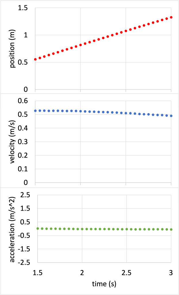
The position graph shows a fairly straight line pointing upward, indicating that the cart increases its position at a steady rate. The velocity graph is also a fairly straight, (approximately) horizontal line, indicating that the velocity stays (about) the same throughout the cart’s motion. The speed at the start is slightly above 0.5 m/s, and the speed at the end is 0.5 m/s. (The speed is not completely constant due to a small amount of friction and air drag.) The acceleration is therefore very close to zero m/s2. This is confirmed by the acceleration graph, which shows a flat line at zero.
Accelerated motion
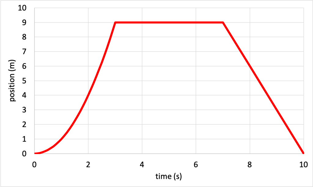
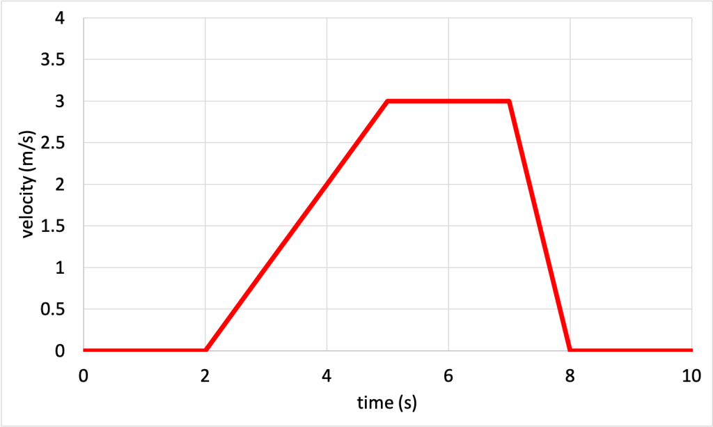
Consider an example that shows all three aspects of acceleration: speeding up, slowing down, and changing direction. As shown in the video below, Dr. Fazzini pushes a cart so that it starts moving up a ramp. As the cart travels up the ramp it slows down. At the point farthest up the ramp it stops for a brief instant, changes direction, and travels down the ramp, speeding up as it gets back to the end of the track.
Position, velocity, and acceleration graphs for this motion are shown in Figure 3.6. (Download this data [XLSX, 12 kB])
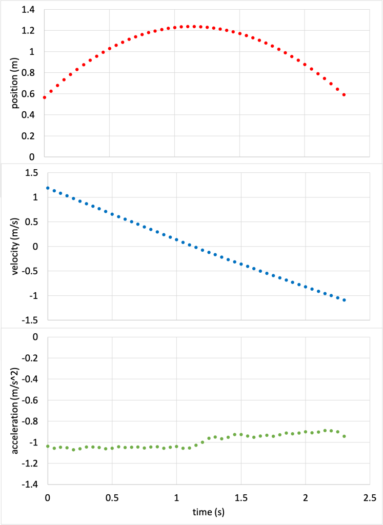
The position graph is a curved trend, resembling a kind of bowl shape, called a parabola. This indicates that the cart changes its position at a decreasing rate as it moves up the ramp, then changes its position at an increasing rate as it moves down the ramp.
The velocity graph is a straight line pointing downward, showing that the velocity decreases at a constant rate. The velocity starts out as large positive numbers, decreases in value, becomes zero briefly when the cart is at the top of the ramp, and then decreases and becomes larger negative values. The speed at the start, after being pushed, is 1.2 m/s, and the speed before being caught after 2.3 s is -1.1 m/s.
Using the equation for acceleration defined above, we can calculate the expected value of acceleration from the velocity data as

In Figure 3.6, the acceleration graph shows a (mostly) straight horizontal line at approximately -1 m/s2, confirming that the acceleration is (mostly) a constant value throughout the motion of the cart. It is worth noting that there is a small change in the average acceleration value after the cart turns around and heads back down the inclined track again. This is because there is a small amount of friction involved. While the cart travels up the ramp, the forces of gravity and friction both act to slow the motion of the cart up the ramp. That is, gravity and friction act together to slow the cart. However, when the cart travels down the ramp, gravity tends to speed up the cart while friction tends to slow the cart, so those two forces are now competing against each other. The result is that the total acceleration of the cart will be slightly smaller in magnitude when traveling down the ramp compared to when the cart travels up the ramp.
The position, velocity, and acceleration graphs tell us a lot about the motion of the cart. The first part, where velocity is negative and acceleration is positive, shows us the period of time when the cart is moving up the ramp and slowing down. An object will slow down when the velocity and acceleration vectors point in opposing directions.
For just an instant of time, the cart stops. This is because the cart must change direction before it rolls back down the hill. The velocity is zero, but the acceleration is still a constant value of -1 m/s2.
For the remainder of the graph, the velocity is positive and the acceleration is positive. This tracks the time when the cart is rolling down the ramp and speeding up. An object will speed up when the velocity and acceleration vectors point in the same direction.
Equations of accelerated motion
The equations to calculate distance and velocity when there is an acceleration present are the most general equations to use in kinematics. They can be used all the time, even when acceleration is zero. But when acceleration is not zero, these equations of motion must be used. The equations are

where  is the displacement, is the acceleration,
  is the time,
  is the initial velocity, and
  is the final velocity of the object.
When acceleration is zero, these equations simplify to

where the first equation is simply a rearranged version of  . (Note that when velocity is constant, it does not make sense to refer to final or initial velocity, but simply velocity.)
The equations of accelerated motion are summarized in the table below:
|
question |
quantity |
equation when acceleration is zero |
equation when acceleration is not zero |
|
how far? |
distance |
|
|
|
how fast? |
velocity |
|
|


Position and velocity graphs
Position, velocity, and acceleration can be plotted in a graph to determine information about the motion of an object. When discussing graphs, we use the terminology “y vs. x” to describe the variable plotted on the vertical axis ( ) as it relates to the variable plotted on the horizontal axis (
 ). Therefore, we would call a graph of position (vertical, or y-axis variable) as it is graphed with respect to time (horizontal, or x-axis variable) a “position vs. time” graph.
Position vs. time graphs
Consider again the person from Figure 3.2, who started at the origin. Say the person moved to the position 4 m to the right of the origin at a constant speed, taking 2 s to arrive at that position. Then they stop and remain still at that position for 2 s. Finally, they move at a constant speed to a position 2 m to the left of the origin at a constant speed, taking 2 s to arrive at the final location. This motion can be graphed with position on the y-axis and time on the x-axis, as shown in Figure 3.7.
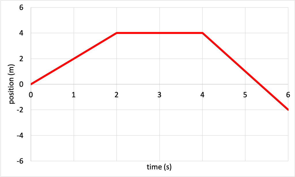
Assuming that the position vs. time graph is composed of straight lines (which is true in Figure 3.7), the slope of each section of the graph is equal to the velocity of the object at that time. For the first 2 s of motion, the person has a velocity of

For the next 2 s of motion, the slope and velocity of the person is zero. For the final 2 s of motion, the person has a velocity of

Velocity vs. time graphs
Just as position can be plotted with respect to time, so can velocity. The velocities calculated above are plotted and shown in Figure 3.8.
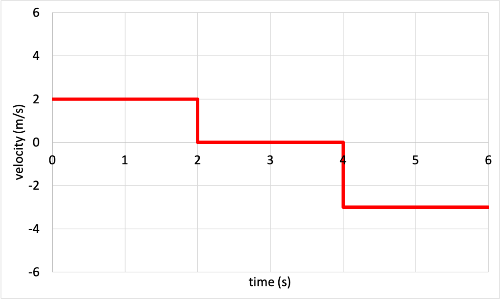
The slope of a velocity vs. time graph is equal to acceleration.
Free fall
The most prevalent source of acceleration in our lives is gravity. Gravity is a force of attraction between masses. It is this attractive force that pulls us down toward the surface of the Earth. That pull produces an acceleration due to gravity, which is equal to 9.8 m/s2 pointing downward. This acceleration is a (mostly) constant value along the surface of the Earth. Because this quantity is used so frequently in physics, it has a special symbol, the lowercase letter g. This symbol (g) refers to the acceleration due to gravity. At times in this textbook this quantity may be referred to as “little g.” This distinguishes it from another quantity, “big g” (G), which is the universal gravitational constant.
Free fall is defined as a situation where gravity is the only force acting on an object. For example, if an object were dropped off the top of a very tall building, free fall would define its motion assuming that there are no other forces such as friction and air drag to slow it down. Free fall is not always a completely accurate way to discuss the motion of an object, but it does a good job in some scenarios, giving us a straightforward way to analyze position, velocity, and acceleration when air drag and friction are negligible.
When analyzing a free-fall situation, we use the equations for distance and velocity when acceleration is present. The value used for acceleration is -9.8 m/s2, as that is the value that comes from gravity. (It is customary to take “up” as positive and “down” as negative. The minus sign signifies that the direction of the acceleration is downward.)
The equations of accelerated motion defined above are used to describe the motion of an object in free fall, using g = -9.8 m/s2 as acceleration.
Consider a ball or other object thrown vertically upward and then caught again at the end of its motion. At the start, the acceleration of the ball points downward and the velocity points upward. Because the two vectors are pointing in opposite directions, the ball will slow down. The ball slows down until it reaches the top of its motion, where it stops just for an instant in time, before moving downward again. Now the acceleration and velocity vectors both point in the same direction, downward. Because the two vectors point in the same direction, the ball will speed up. The ball speeds up until it is caught and ends its motion. The acceleration is constant throughout the motion of the ball.
The last sentence of the previous paragraph bears repeating: the acceleration is constant throughout the motion of the ball. Gravity is constant, and it never turns off. The ball may instantaneously stop at the top of its motion, but that’s because gravity is pushing down on the ball, and as it’s moving upward it slows down and must change its direction before coming back down to the Earth. The acceleration due to gravity is -9.8 m/s2 the entire time the ball is moving. It is a constant value that never changes.
People often find it difficult to accept that the acceleration is not zero at the very instant that the velocity is zero. However, during the flight, the velocity is always changing. Even when the ball reaches the top of its flight, the velocity is still changing. It just happens to be changing through zero (from positive to negative). If the acceleration was zero at any time during the flight, there would have to be at least two points on the velocity graph that have the same value. Since this never occurs, the acceleration cannot be zero at any time while the ball is in the air. This was also the case for the cart that was pushed up the ramp and then came back down. In Figure 3.6, it is clearly seen that the acceleration is never zero (even when the cart momentarily stops at the top of its climb).
Further reading
- Penny Drop (MythBusters season 1, episode 4, 2003) – This episode of MythBusters debunks the myth that dropping a penny from the top of the Empire State Building would destroy the sidewalk and kill any pedestrians unlucky enough to stand at the base of the building.
Practice questions
Conceptual comprehension
- If you go for a drive, recall that the odometer on your car measures the path that the car has driven. Using a piece of string and a map, describe how you could go about calculating the displacement of the car for that excursion.
Numerical analysis
- A person walks 30 m east, then turns around and walks 15 m west. Calculate the person’s path. Then, calculate the person’s total displacement.
- An elevator starts at the ground floor and goes up to the fifth floor, then comes back down to the third floor. Calculate the elevator’s path. Then, calculate the elevator’s total displacement. (Use units of floors in your calculations.)
- A skier starts at the top of a hill, descends 500 m downward along the slope of the hill, climbs 100 m back upward along the slope of the hill, then skis an additional 400 m downward along the slope of the hill. Calculate the skier’s path along the slope of the hill. Then, calculate the skier’s total displacement along the slope of the hill.
- A boat moves 10 km downstream in a river flowing at 5 km/hr. Later, the boat returns to its starting point by moving 10 km upstream. Calculate the boat’s path. Then, calculate the boat’s total displacement.
- A car travels east to west from point A to point B, covering a distance of 200 km in 2 hr. Calculate the car’s average speed. Then, calculate the car’s average velocity. (Use units of m/s in your calculations.)
- A bird flies 2 km north in 20 min and then returns 2 km south in 15 min. Calculate the bird’s…
- …instantaneous speed as it flies north.
- …instantaneous speed as it flies south.
- …average speed for its entire journey.
- …average velocity for its entire journey.
- Draw a position vs. time graph and a velocity vs. time graph for an object moving with a steady pace in the positive direction, and then stopping and staying still for several moments.
- Draw a position vs. time graph and a velocity vs. time graph for an object that starts at rest for several moments, then moves at a constantly increasing speed for the next several moments.
- Draw a position vs. time graph and a velocity vs. time graph for an object that speeds up at an increasing rate, travels at a constant rate for a few moments, and then slows down until it stops.
- Describe the motion needed to generate the position vs. time graph shown in Figure 3.9.
- Describe the motion needed to generate the velocity vs. time graph shown in Figure 3.10.
- A train travels a distance of 500 m in 20 s at a constant speed. Calculate the speed of the train.
- A car starts from rest and accelerates at a rate of 2 m/s2 for 5 s. Calculate the car’s final velocity. Then, calculate the distance the car traveled during the 5 seconds.
- An object is thrown vertically upward with an initial velocity of 20 m/s and travels in free fall. Calculate how high the object will go.
- An object falls freely from a height of 40 m. Calculate the amount of time it took the object to hit the ground. Then, calculate its velocity just before it hits the ground.
Path describes the total distance that an object travels as it moves from one point to another, measured along its trajectory. It is a scalar quantity. (symbols: d, x [for horizontal path], y [for vertical path], unit: m)
A scalar quantity is a variable that can be conveyed with a numerical quantity indicating magnitude or strength.
Displacement describes the straight-line distance from one point to another. Displacement is a vector quantity. (symbols: Δd [for general displacement], Δx [for horizontal displacement], Δy [for vertical displacement]. unit: m).
A vector quantity is a variable that must be conveyed with both a numerical quantity (indicating magnitude or strength) and a direction.
Speed is the scalar quantity that describes the rate at which an object changes its position. Speed is equal to position divided by time. (symbols: s, |v|, unit: m/s)
Velocity is the vector quantity that describes the rate at which an object changes its position. Velocity is equal to displacement divided by time. (symbol: v, unit: m/s)
Acceleration quantifies the rate at which an object changes its velocity. (symbol: a, unit: m/s^2)
Physics is a branch of science that focuses on the fundamentals of the workings of our universe.
The net force is the vector sum of all forces acting on an object.
Gravity is the attractive force experienced by objects of mass. It is one of the four fundamental forces.
A force is a push or a pull that causes an object to change its motion. More fundamentally, force is an interaction between two objects. (symbol: F, unit: N)
Mass is a property of physical objects that relates to resistance to changes in motion: inertia. (symbol: m, unit: kg)
Free fall is defined as a situation where gravity is the only force acting on an object. Forces such as friction and air drag are ignored and assumed to be equal to zero. The acceleration of an object in free fall is defined by the acceleration due to gravity (g).
