19. Vibrations and waves
Summary
Many aspects of our lives are dictated by waves. Light waves are used to transmit Wi-Fi and cellular signals, sound waves are used to communicate with others, and even the motion of a pendulum that keeps time in a grandfather clock has wave properties. There are many periodic events in our lives that occur at repeatable time intervals: sunrises, moon phases, seasons, heartbeats, and more.
This chapter will discuss different waves and wave properties, and start a fascinating conversation about waves that will unlock the mysteries of sound and light in chapters to come.
Vibrations and waves
A vibration is a periodic back and forth motion that remains fixed in one location. Examples of vibrations include a swing moving back and forth (like a pendulum) or a mass bobbing up and down on a spring. The video below demonstrates this periodic back and forth motion using the example of a swing set. (While the swing moves back and forth, this periodic motion does not propagate through space. Therefore, it is an example of a vibration.)
A wave is a traveling vibration that transfers energy from one place to another. There are many different types of waves: light waves, sound waves, water waves, gravitational waves, seismic waves, and more.
The term periodic oscillation refers to the types of motion that waves make. This is a repeating pattern that causes many wave properties. A wave is periodic motion that gives rise to a variation in some value (intensity, energy, pressure, or some other property) over time as the wave property propagates through space. The video below demonstrates both the time-varying and space-varying properties of a wave as it travels. It shows that, at a single point in space, the wave properties vary with time. It is also possible to see how a wave varies in space at a single snapshot in time.
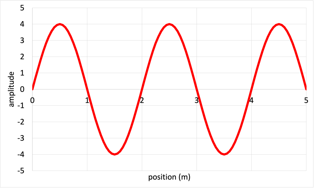
In the video above, and in many types of periodic motion, waves may look like a “squiggle” that moves up and down in space and time. Formally, this particular “squiggle” shape, shown in Figure 19.1, is known as a sinusoid. This comes from the trigonometric function “sine.” While we will not make use of any trigonometric functions in this textbook, the shape of a sine (or sinusoidal, meaning “sine-like”) wave appears often enough to informally define it here. The wave shown in Figure 19.1 depicts the value of a wave as it moves through space at a single snapshot in time.
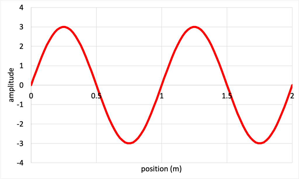
Each of the high points on the wave is known as a peak or crest. Each low point of the wave is a valley or trough. The center position is known as the equilibrium value of the medium. This would show us the undisturbed value of the property (energy, intensity, pressure, or another property) of the medium; in other words, the value that a particular property of the medium would have if it was at rest.
Wave properties
In order to characterize a wave, we need to be familiar with the terms used to describe waves. Wave amplitude describes the maximum displacement from the equilibrium position. In other words: how far away from the equilibrium position are the crests and troughs? Depending on the wave, the amplitude could describe energy, intensity, or even just height. (For example, the amplitude of a mass bobbing up and down on a spring could represent length. The amplitude of a swinging pendulum may represent degree from the vertical.) So we will not necessarily define one particular unit for amplitude, as it could be describing one of many physical parameters.
The video below shows an animation of a wave where the amplitude gradually increases over time.
The wavelength of a wave describes the shortest distance between two identical repeating points on a wave. Wavelength is most easily measured from crest to crest (or from trough to trough) on a wave. More precisely, wavelength is the distance between subsequent repeating points on the wave (where the wave has the same value and the same slope). The requirement of the same slope is important, otherwise if two adjacent points with just the same value are selected (without paying attention to slope), a value less than the wavelength will be measured. (This is why it is simpler to measure wavelength from crest to crest or from trough to trough.) Figure 19.2 shows a few possible ways to measure wavelength using this definition.
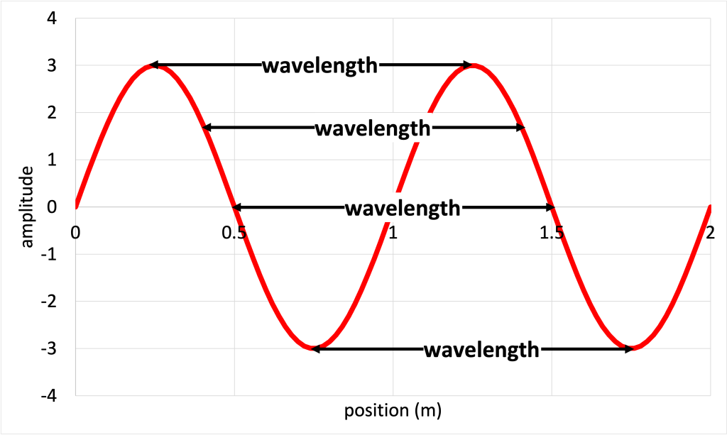
The symbol for wavelength is the lowercase Greek letter lambda ( ). It has units of distance: meters or centimeters.
The video below shows an animation of a wave where the distance between adjacent wave crests gradually decreases over time.
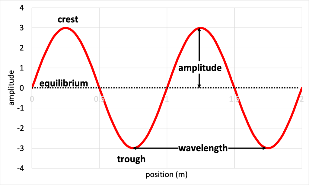
Figure 19.1 was annotated to include the crest, trough, equilibrium, amplitude, and wavelength. This is shown in Figure 19.3.
The period of a wave describes how long it takes for one complete oscillation (out and back motion) to occur. An oscillation, simply put, is a complete motion from crest to crest or from trough to trough. (More accurately, an oscillation is the time it takes for a particle to return to its initial position and be moving in the same direction. As with wavelength, it is important not to ignore the second requirement in this definition!) In a pendulum, an oscillation relates to the amount of time it takes for the pendulum to swing out and back again. The symbol for period is the capital letter T, and the unit is seconds.
Frequency describes how many wave oscillations occur per second. Frequency is represented by the symbol  and is measured in the unit hertz (Hz). One hertz is equal to one oscillation divided by a second. Frequency and period are related by the equation

In other words, frequency is equal to one divided by the period. The higher the frequency of oscillation, the faster the wave squiggles in time, and the shorter each period will be.
Wave speed describes the speed at which a wave moves. We know that speed is equal to distance divided by time. In this case, the distance described by the wave is the wavelength, and the time is described by the period. This means that the wave speed is equal to wavelength divided by the period. In equation form,

Or, we can rewrite the equation to say that wave speed is equal to wavelength times frequency,

If wave speed is constant, then this equation can tell us the relationship between wavelength and frequency.
Types of waves
Waves tend to be characterized by the motion that the wave itself makes compared to how the wave travels through space.
Longitudinal waves
In a longitudinal wave, the oscillations (back and forth motion) of the wave travel in the same direction as the wave itself. The video below shows an animation of many particles oscillating in a longitudinal wave. The motion of the particles is parallel to the motion of the wave itself.
Sound waves are examples of longitudinal waves. This type of wave will be explored in more detail in the next chapter of this textbook.
Transverse waves
In a transverse wave, the vibrations of the wave move perpendicularly to the direction of motion of the wave. In the video below, a transverse wave is animated as it travels through time and space. A red point on the wave demonstrates the motion of oscillation, which is perpendicular to the direction that the wave propagates.
Water waves
There are also some waves that are neither purely longitudinal nor purely transverse. Water waves in the ocean, for example, are usually a mixture of both longitudinal and transverse. There is both up-and-down and side-to-side motion in ocean waves.
The video below shows an animation of a water wave. Each point in the wave can be seen moving with both parallel and perpendicular motion compared to the motion of the wave itself.
Traffic waves
It might be strange to think of traffic as a wave, but you should think about it next time you’re at a traffic light. At a red light, cars stop and line up. When the light turns green, the motion of the cars will be forward, but the direction that the information in the wave moves is backward. The first car in line moves forward, and then the car behind that one moves, and the car behind that one, and so on.
The video below is an animation of a simulation of cars (each one is represented as a square) stopped at a red light. When the light turns green, each car subsequently starts moving. When a car is red, that means it has started moving. The position of the red square, representing the information transmitted by the wave, moves backward, even though the cars move forward.
Torsional waves
Another type of wave is known as a torsional wave. This is a type of twisting back and forth in a periodic manner. The video below shows a mass twisting back and forth in a torsional wave.
A torsional wave is what caused the Tacoma Narrows Bridge to collapse in 1940. Winds blowing across the bridge created and amplified the torsional wave in the bridge, which eventually overcame the strength of the structure, causing its collapse.
Interference
We know that two objects of matter cannot occupy the same space at the same time. Waves are energy, not matter, so they can exist in the same place at the same time. When waves overlap with each other they interfere. That is, the value of one wave at that point adds to the value of the second wave. The total amount of energy present is equal to the sum of those two values.
If two waves interfere where the crest overlaps with crest, and trough overlaps with trough, then the situation is called totally constructive interference. The result is a wave with greater overall amplitude than either one individually. If the two waves have identical amplitudes, the constructive interference will yield a wave with twice the amplitude. The video below shows an animation of two wave pulses interfering constructively.
If two waves interfere where crest overlaps with trough, and trough overlaps with crest, then the situation is called totally destructive interference. If the two waves have the same amplitude, then if we sum up the contributions of each wave, they cancel out. The result is a wave with zero amplitude. This condition of destruction is temporary: as the waves continue to propagate, as they stop overlapping with each other, the interference will end. The video below shows an animation of two wave pulses interfering destructively.
It is also possible to have many other types of interference that are neither purely constructive nor purely destructive (the interference may be “partially constructive” or “partially destructive”). The video below shows an animation of the interference of two waves, which is neither necessarily constructive nor destructive.
Interference happens all the time: when pebbles are dropped in a pond, when light waves interact, and when sound waves come together. The interference of light waves was used to prove that the speed of light is constant, which was one of the foundational experiments of the 19th century.
Standing waves
Standing waves are waves that oscillate in time but that do not move at all in space. They occur due to interference between two waves that have equal amplitude and frequency that travel in opposite directions.
Two fixed ends
In the video below, Dr. Pasquale generates standing waves in a coiled rope by shaking one end up and down. Both ends of the coiled rope are held firmly into place. These are known as fixed ends as they are physically unable to move. This creates one wave, which reflects off of the back end of the coiled rope and travels back toward her arm. By shaking at the right frequency, the two waves: the forward wave and the backward wave: will interfere just right to create a standing wave.
Locations on a standing wave that are fixed are known as nodes. Locations where the wave oscillates between minimum and maximum values are called antinodes. These are depicted in Figure 19.4.
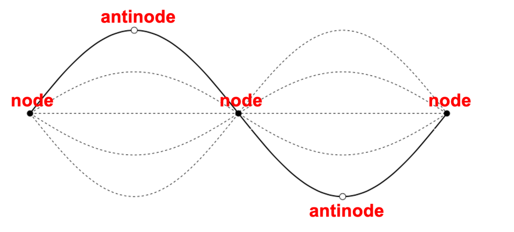
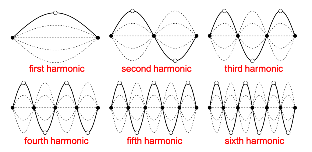
Each standing wave that can be generated is known as a harmonic. When there are two fixed ends, each end of the standing wave is a node. The first harmonic is the wave with one antinode and two nodes. The first harmonic is also sometimes referred to as the fundamental mode. The first harmonic represents one half of a wavelength of the full wave (in other words: the distance between two successive nodes is half of a full wavelength).
The second harmonic has two antinodes and three nodes as shown in Figure 19.4. The second harmonic represents an entire wavelength of the full wave. The third harmonic has three antinodes and four nodes, and represents one and a half wavelengths. The information for the first six harmonics (with two fixed ends) is given in the table below.
|
harmonic |
antinodes |
nodes |
wavelengths |
|
1 |
1 |
2 |
0.5 |
|
2 |
2 |
3 |
1 |
|
3 |
3 |
4 |
1.5 |
|
4 |
4 |
5 |
2 |
|
5 |
5 |
6 |
2.5 |
|
6 |
6 |
7 |
3 |
The first six harmonics are shown graphically in Figure 19.5.
For a given medium (for example, the coiled rope used in the video above), the wave speed of a standing wave will be constant. Because the wavelength of each standing wave is related to the harmonic, the frequency will also be related to the harmonic number.
As the harmonic number increases, so does the frequency. In fact, the frequency of a harmonic is related to the number of the harmonic and the frequency of the first harmonic. In equation form: the frequency of the nth harmonic is equal to  , the harmonic number, times the frequency of the first harmonic:

where  is the frequency of the first harmonic.
Non-fixed ends
It is possible for a standing wave to have, for example, one fixed end (a node), and one end that is free to move up and down. (It is assumed that the ring slides up and down on the post with negligible friction.) This is shown in Figure 19.6.
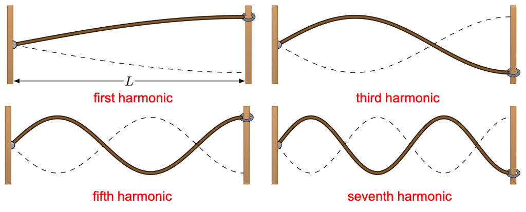
In this case, the fixed end of the standing wave is a node, and the free end of the standing wave is an antinode. Whereas standing waves with two fixed ends support multiples of half wavelengths, standing waves with one open end only support multiples of odd fourths of wavelengths. Because of this configuration, only odd harmonics are generated. The information for the first six harmonics (with one fixed end) is given in the table below.
|
harmonic |
antinodes |
nodes |
wavelengths |
|
1 |
1 |
1 |
0.25 |
|
3 |
2 |
2 |
0.75 |
|
5 |
3 |
3 |
1.25 |
|
7 |
4 |
4 |
1.75 |
|
9 |
5 |
5 |
2.25 |
|
11 |
6 |
6 |
2.75 |
From this table, we can see that in each length  between supports of the rope, there are
  wavelengths present, where is the harmonic number. Solving for wavelength, we can see that

As discussed with standing waves with two fixed ends, the wave speed of a standing wave will be constant (assuming the medium stays the same). Because the wavelength of each standing wave is related to the harmonic, the frequency will also be related to the harmonic number. In fact, the same relationship between the harmonic frequency and first harmonic exists with standing waves with one fixed end! That is,
where is the frequency of the first harmonic.
Just as it is possible to have transverse standing waves (depicted in Figures 19.4, 19.5, and 19.6), it is also possible to create longitudinal standing waves (for example, from sound waves). As with transverse standing waves, when a longitudinal wave is created in a cavity (such as a pipe or a musical instrument), any time there is a closed end, there will be a node of the longitudinal wave. Any time there is an open end, there will be an antinode of the longitudinal wave. This is how sound waves are generated in many musical instruments.
The first three harmonics of a longitudinal standing wave generated in a pipe with one closed and one open end are shown in Figure 19.7. The pipe is filled with water (depicted in gray in the figure), and the water level creates a closed end. The black dots in this figure represent air molecules. At the locations without the arrows, the molecules essentially do not move; these are the standing wave nodes. The dots shown with the arrows indicate the locations where the molecules vibrate with their greatest amplitude; these are the standing wave antinodes. The solid arrows indicate that air molecules at those points are at a maximum at one snapshot in time (similar to the solid lines shown in Figure 19.5 and Figure 19.6). Note that two successive antinodes will have the particles on opposite sides of the equilibrium position. The dashed arrows show the same thing half a period later (similar to the dashed lines shown in Figure 19.5 and Figure 19.6).
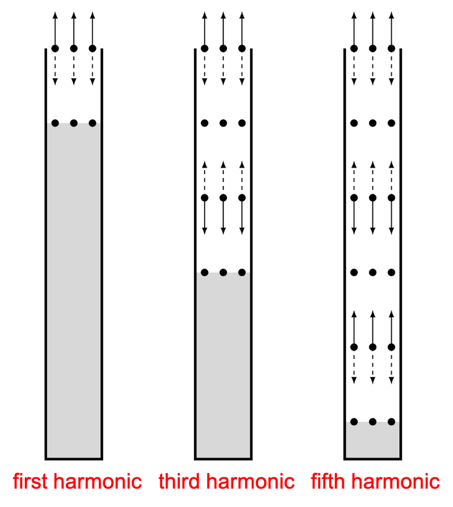
In this particular figure (Figure 19.7), the wavelength of each wave remains fixed; the length (distance between the open end of the pipe and water level) is changed to support the standing wave. If the wavelength of the standing wave is known, the length can be calculated as

The Doppler effect
Have you ever noticed that when an ambulance or police car drives by, the pitch of the sound of the siren seems to change? This is due to the Doppler effect. The Doppler effect is the perceived change in frequency of a sound wave as heard by an observer when either the source of the sound or the observer moves through the medium.
When a wave is traveling at a certain speed relative to an observer, the wavefronts become bunched up in the direction of motion. This is because the source moves toward the previously emitted pulse before emitting the next pulse. This shortens the wavelength and (since the wave speed is constant) increases the frequency. Frequency and pitch are related in sound waves, which is why a siren sounds higher in pitch when an ambulance is approaching your location.
In a similar manner, as a wave travels away from the observer, the wavefronts are spread farther apart. This increases the wavelength and decreases the frequency. This means that a siren sounds lower in pitch when it is moving away from your location.
An animation of the Doppler effect is shown in the video below. The wavefronts are compressed in the direction of travel, and spread out in the direction opposite travel.
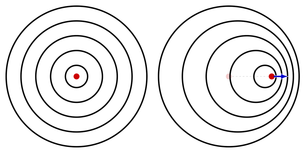
Figure 19.8 (left) shows the wavefronts of a stationary wave, where all wavelengths are equal in all directions. Figure 19.8 (right) shows the wavefronts of a moving wave, where the Doppler shift is evident.
If, instead of the wave (source) moving relative to the observer, the observer moves relative to a stationary source, the results of the Doppler effect are qualitatively the same (a change in perceived pitch of the sound), but are not numerically the same. There is an equation that can be used to determine the exact numerical change in perceived frequency of the sound wave:

where  is the perceived frequency heard by the observer,
  is the original frequency emitted by the source,
  is the speed of sound at that temperature and in that medium (the speed of sound will be formalized in the next chapter of this textbook),
  is the speed of the observer with respect to the medium, and
  is the speed of the wave source with respect to the medium.
While this equation may look complicated, it is really just a compact way of dealing with all of the possible ways (in a one-dimensional scenario) that the source and observer can move relative to each other and through the medium. Note that when you are using this equation, if either the source or the observer approaches the other, the frequency increases. If the source or observer moves away from each other, decreases.
All of the different scenarios including this Doppler equation are outlined in the table below.
|
scenario |
equation |
|
observer moves toward a stationary source |
|
|
observer moves away from a stationary source |
|
|
source moves toward a stationary observer |
|
|
source moves away from a stationary observer |
|
|
source and observer both move toward each other |
|
|
source and observer both move away from each other |
|
|
source chasing the observer |
|
|
observer chasing the source |
|


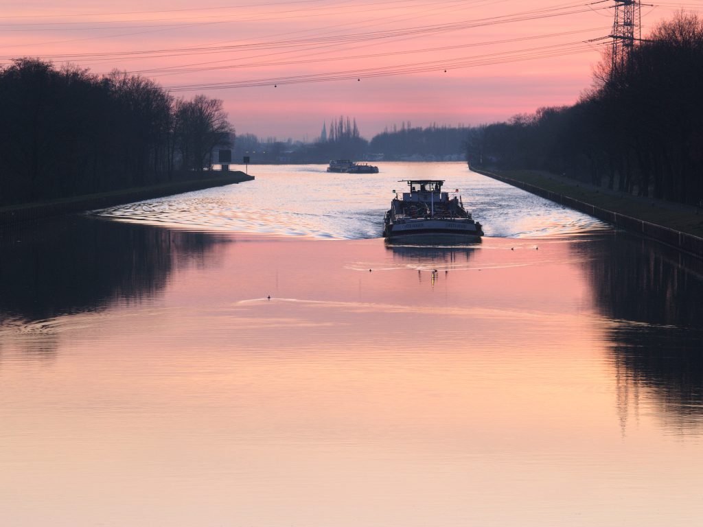
Depending on the wave, the speed of motion can have profound applications due to the Doppler effect causing the wavefronts to bunch together. In a boat, water is the physical medium in which waves propagate. If we drop a pebble into a pond, the ripple pattern is even and uniform.
If, however, we continuously drop pebbles while in motion, the Doppler effect will cause the wavefronts to bunch together. At a certain point, when the pebble moves at the same speed as the speed of the water waves, a wake will form. This happens with boats, which generate bow and stern waves when they travel across water faster than the disturbance they create would travel across the water. Figure 19.9 shows V-shaped waves called bow waves generated by a barge and several ducks.
For sound waves, when the speed of an object travels faster than the speed of sound, this disturbance creates a sonic boom. This is a shockwave created due to the overlapping of wavefronts at a speed faster than the air can meaningfully respond to the changes in pressure caused by the wave. This compresses the air and creates the shock wave we call a sonic boom.
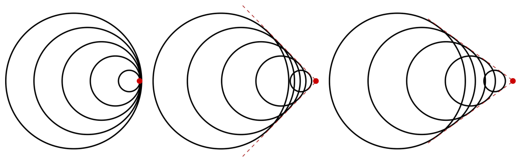
A sonic boom travels in a three-dimensional cone shape whose angle corresponds to the exact speed of the supersonic object. The faster the motion of the object, the smaller the angle of the cone becomes. This is demonstrated in Figure 19.10, where an object is depicted traveling at exactly the speed of sound (left), creating a sonic boom normal to the direction of motion. An object moving faster than the speed of sound (middle) has wavefronts that overlap at an angle, and an object moving even faster (right) has wavefronts that overlap at a smaller angle relative to the direction of motion of the object.
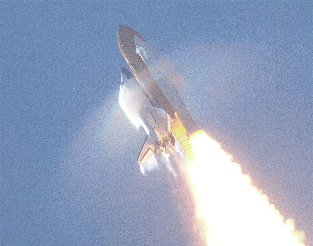
The shockwave generated by a space shuttle orbiter is shown in Figure 19.11.
Further reading
- Acoustics and vibrations animations – This website contains animations of many different types of waves (longitudinal, transverse, etc.).
- Circular harmonics – Animations of circular harmonics, which are the waves that are created on a circular membrane, such as a drumhead.
Practice questions
Numerical analysis
- Use the graph in Figure 19.12 to calculate the…
- …amplitude.
- …wavelength.
- …wave speed, assuming the frequency is 4 Hz.
- Calculate the frequency of a wave that completes 10 oscillations in 2 seconds.
- If a wave has a period of 0.5 s, calculate its frequency.
- A wave with a wavelength of 2 m travels through a medium at a speed of 20 m/s. Calculate the frequency of the wave.
- If a wave has a frequency of 100 Hz and a wavelength of 0.1 m, calculate its wave speed.
- A standing wave has a first harmonic frequency of 440 Hz. Calculate the frequency of the…
- …second harmonic.
- …third harmonic.
- A standing wave has a third harmonic frequency of 900 Hz. Calculate the frequency of the first harmonic.
- The first harmonic of a standing wave has a wavelength of 2 m. Calculate the length of the string used to generate the standing wave.
- A standing wave on a guitar string that is 30 cm long has three nodes. Calculate…
- …the harmonic of the standing wave.
- …the wavelength of the wave.
- …the frequency of the wave, assuming the wave speed is 340 m/s.
- A standing wave on a rope that is 1.2 m long has five antinodes. Calculate…
- …the harmonic of the standing wave.
- …the wavelength of the wave.
- …the frequency of the wave, assuming the wave speed is 8 m/s.
Hands-on experiments
- If you have a SlinkyTM, use it to generate a longitudinal wave. Then use it to generate a transverse wave.
- Fill a shallow tray or a baking dish with water. Drop small objects like coins or pebbles into the water to create ripples. Observe how these waves move, reflect off the edges, and interfere with each other. You can also use a small stick (or your finger) to generate waves by tapping the water’s surface.
A vibration is a periodic back-and-forth motion that remains fixed in one location.
A wave is a periodic oscillation that transfers energy from one place to another.
Energy is defined as the capability of an object (or collection of objects) to do useful work. (symbol: E, unit: J)
A sound wave is a longitudinal wave that is caused by vibrations in air pressure between two points.
Intensity describes the amount of energy per unit of area that reaches a certain location every second (unit: W/m^2)
Pressure defines the amount of force applied over an area of a substance. (symbol: P, unit: Pa)
Wave amplitude describes the maximum displacement from either side of the equilibrium position.
The wavelength of a wave describes the shortest distance between two identical repeating points on a wave. (symbol: λ, unit: m)
The period of a wave describes how long it takes for one complete oscillation to occur. (symbol: T, unit: s)
Frequency describes how many oscillations occur per second in a wave. (symbol: f, unit: Hz)
Speed is the scalar quantity that describes the rate at which an object changes its position. Speed is equal to position divided by time. (symbols: s, |v|, unit: m/s)
In a longitudinal wave, the oscillations of the wave travel in the same direction as the wave itself.
In a transverse wave, the vibrations of the wave travel perpendicular to the direction of motion of the wave.
Interference is the phenomenon that occurs when two waves overlap. The total amount of wave energy present at a point is equal to the sum of each individual wave's energy at that point.
A standing wave is a wave that oscillates in time but that does not move in space. Standing waves occur due to interference between two waves that have equal amplitude and frequency that travel in opposite directions.
The Doppler effect is the perceived change in frequency of a sound wave as heard by an observer when there is motion between the observer and the source.
Temperature defines the average kinetic energy of an object. It quantifies the “hotness” or “coldness” of something. (symbol: T, unit: °C or K)
