32. Quantum physics
Summary
The Bohr model of the atom
Earlier in this textbook, we discussed atomic models. From Democritus to Thomson to Rutherford, we learned how each of the atomic models came to be, and what experimental evidence led to changes in how we understand atoms over the past several centuries.
As discussed earlier in this textbook, the emission spectrum of an element is the collection of frequencies of light emitted via deexcitation of excited electrons in the gaseous form of that element. If instead of measuring the light emitted from the gas, we shine a continuous spectrum of light onto that gas, those same frequencies can cause excitations that remove light and produce dark lines in the continuous spectrum. This is called an absorption spectrum.
While these spectra have been observed since the early 1800s, it was not until 1885 that Johann Balmer discovered a simple empirical formula that correctly calculated the visible wavelengths from the frequencies observed in the spectrum of hydrogen. (Hydrogen, the simplest atom, has an emission spectrum with fewer lines and more order than any other elemental atom.) The series of visible lines later became known as the Balmer series in his honor. Although Balmer did not know why his formula worked, his formula was able to correctly predict the existence of other spectral lines (in the non-visible region of the electromagnetic spectrum) that were yet to be observed.
It was generally believed that atomic spectra were clues to the structure of atoms in much the same way that particular resonant frequencies are related to a musical instrument.
In 1913, Danish physicist Niels Bohr made use of Ernest Rutherford’s nuclear model of the atom and put forth a new model of the atom and found that he could derive Balmer’s formula using a blend of classical physics and quantum assumptions that Bohr made. (These assumptions turned out to be correct, but at the time, Bohr had no basis for making them.) This model is known as the Bohr model of the atom.
In his model of the hydrogen atom, Bohr proposed that the electron was held in a circular orbit around the nucleus (a single proton) by the electric force, analogously to a planet held in orbit around its sun by gravity. However, unlike the planet, which can orbit at any arbitrary distance, the electron could only orbit at certain discrete distances with only certain allowed energies. This is where the quantization concept enters the picture. Bohr’s model of electrons orbiting atoms in discrete orbits given by energy levels was prompted by the measurements of atomic emission spectra that exhibit discrete frequencies.
The classical model of an electron orbiting a nucleus would indicate that the electron is accelerating. (As discussed, an object that moves in a curved path necessarily accelerates.) Maxwell’s theory of electromagnetism states that accelerating electrons emit light (which was discussed in chapter 30 in this textbook in the context of the generation of x-rays). Because Bohr’s model predicts that electrons travel in a curved path, it would be reasonable to expect that those electrons would emit light. However, it is known that electrons traveling in orbits do not emit light. Bohr simply asserted that they do not radiate while traveling in these atomic orbits, without giving an explanation for this discrepancy between his model and observed reality. However, Bohr’s model did account for electrons making a “quantum leap” from one allowed orbit to another, by either absorbing or emitting a photon that has energy equal to the energy difference between the two orbits.
Electron waves
The shortcomings of a purely “planetary” and particle-like model of electrons can be explained by the wave nature of electrons. Recall that the double-slit experiment experimentally demonstrated that electrons exhibit wave-like behavior. That’s true when electrons are orbiting an atom as well as when electrons travel freely through space.
Each electron will form a standing wave as it moves about the nucleus. Only waves that have a particular radius, given by the constructive interference of waves, can be supported in shells around the atom. This video below shows an analogy of how this works. If each shell is constituted by an integer value of the electron’s wavelength, which would support constructive interference, then those shells have very well-defined sizes. This is analogous to the standing waves we discussed previously in this textbook.
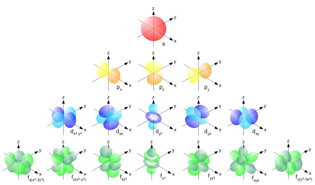
In fact, electron waves are more complicated than this, but this conceptual understanding helps to describe the quantum picture of electrons, and addresses the drawbacks of the classical model of electron orbits. The actual electron orbitals take on very bizarre shapes that include lobes and donuts in highly directional orientations based upon the solutions to an equation that will be discussed later in this chapter. Figure 32.1 illustrates some of these orbital shapes.
Quantum mechanics
Quantum mechanics is the study of mechanics (the description of the motion of physical objects of matter) when things become so small that classical physics breaks down and stops working adequately. Quantum objects have three major differences from classical objects.
- The properties of quantum objects (such as energy and momentum) appear in discrete, quantized values.
- Quantum objects exhibit wave-particle duality.
- Quantum objects have fundamental limits to the degree of precision that can be obtained when measuring certain quantities, given by the uncertainty principle.
How do we measure quantities using quantum mechanics? When considering a particle in a classical situation, the future behavior of the particle can be obtained with absolute certainty using Newton’s laws (particularly  ). When considering any distribution of charges or currents, the electric and magnetic fields can be found using Maxwell’s equations. At the heart of quantum mechanics is an equation proposed by Austrian physicist Edwin Schrödinger in 1926. This equation (known as the Schrödinger equation) is the means by which the future behavior of quantum particles is predicted. It should be mentioned that Newton’s laws, Maxwell’s equations, and the Schrödinger equation cannot be derived from basic principles because they are basic principles. The validity of Newton’s laws, Maxwell’s equations, and the Schrödinger equation comes from their ability to make predictions consistent with experimental observations.
In the search for the Schrödinger equation, there are certain properties the equation is expected to have.
- It needs to be consistent with conservation of energy:
 .
. - It has to be consistent with de Broglie’s hypothesis of the wave nature of matter
 .
. - It needs to give results that are consistent with the observed experimental results.
While it is possible to generate equations that are consistent with the first two points (obeying conservation of energy, and being consistent with de Broglie’s matter wave hypothesis), only the Schrödinger equation (presented below) satisfies all three of these points as it also gives results that are consistent with known experimental data. (Source: Krane, Kenneth S., Modern Physics. John Wiley, 1983.)
We now return to the question of what is oscillating when it comes to de Broglie’s matter waves. What we find in quantum mechanics is that objects can be described with a mathematical quantity known as the wave function, denoted by the Greek letter psi ( ). It is interesting to note that de Broglie and even Schrödinger did not know how to interpret the wave function. It was Max Born, a German physicist, who in 1926 found that the wave function was related to the probability of finding the particle in a particular region of space in a particular time frame. (More accurately, Born found that it was the magnitude of the square of the wave function that provided these probabilities.) Furthermore, the wave function could be used to calculate the probability of the outcome of different measurements that can be made on a quantum object. For example, the wave function can be used to determine the probability that a quantum particle (such as an electron) will have a particular energy or momentum within a certain range. As bizarre as it may sound, it is waves of probability that are actually oscillating!
It is important to point out that while the Schrödinger equation will be shown below for demonstration purposes, it is not expected that you will use this equation at all, as it is extremely complicated! The mathematics in this equation goes way beyond the math that you are expected to have learned at this stage. In a way, that’s the point: quantum mechanics is a very difficult model of physics that we don’t use on the macro scale because it is not necessary! Why use this complicated equation when we can use simple equations like and get the same results?
Schrödinger’s equation is
![$$[\frac{-\hbar^2}{2m} \nabla^2 + U]\psi = i\hbar \frac{\partial \psi}{\partial t}.$$](https://cod.pressbooks.pub/app/uploads/quicklatex/quicklatex.com-0a345429a15471688cb88e465176862d_l3.png "Rendered by QuickLaTeX.com")
The left-hand side of the equation contains terms that have to do with how the wave function changes in space. The first term essentially deals with the kinetic energy and the second term deals with the potential energy. The right-hand side of the equation contains terms that have to do with how the wave function changes in time and relates to the total energy of the object. We see Planck’s constant divided by two pi ( ) twice.
  is the mass of the quantum object. The upside-down triangle (
 ) and squiggly d (
 ) are calculus operators.
  is the square root of negative one, and leads to wave properties when doing calculus.
To reiterate, instead of obtaining exact values of energy, position, and momentum, like we can calculate in classical physics, the wave function provides us with probabilities. A wave function for an electron orbiting a nucleus will give us the probability of finding an electron existing at any one orbital state around the nucleus of an atom.
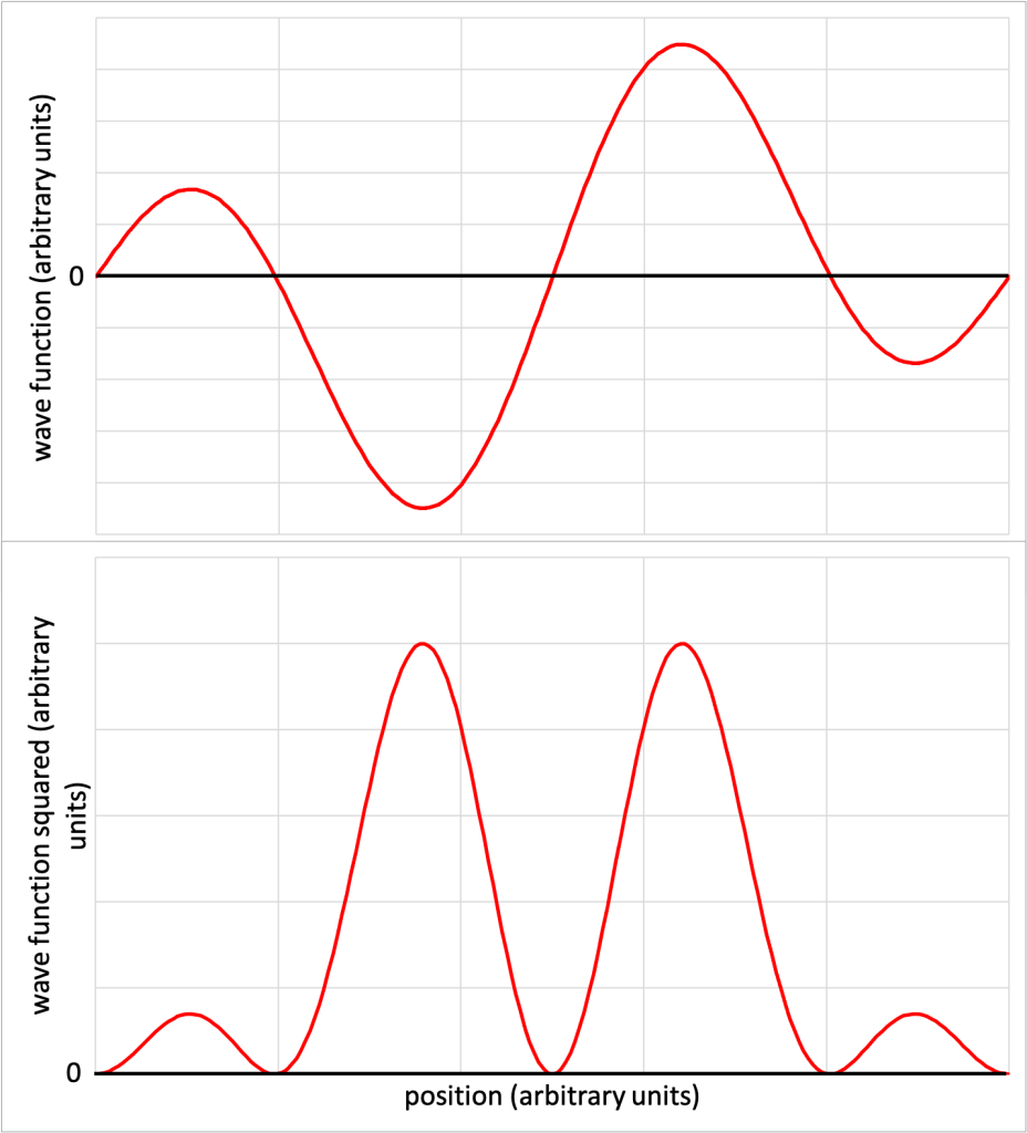
To illustrate this idea, Figure 32.2 shows a contrived wave function (Figure 32.2, top) and the square of the wave function  (Figure 32.2, bottom). The tall regions near the center of the graph indicate a high probability of finding the particle slightly off center of the region. The smaller peaks indicate that the particle has a lower probability of being found near the outer edges of the region. The five locations where is zero indicate the particle will never be found at those locations.
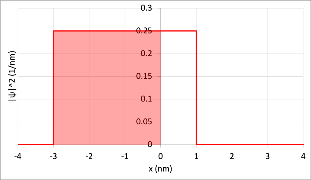
To solve for the probability of finding a particle within a particular range of values, it’s necessary to calculate the area under the curve of the wave function squared within that range. To demonstrate this, consider Figure 32.3, which shows a simplistic wave function (Figure 32.3, top) and the square of that wave function (Figure 32.3, bottom). (Download this data [XLSX, 9 kB]) Note that this particular wave function does not correlate to any realistic particle. Instead, it has been contrived to make the mathematics of solving under the curve possible without using calculus or other advanced math.
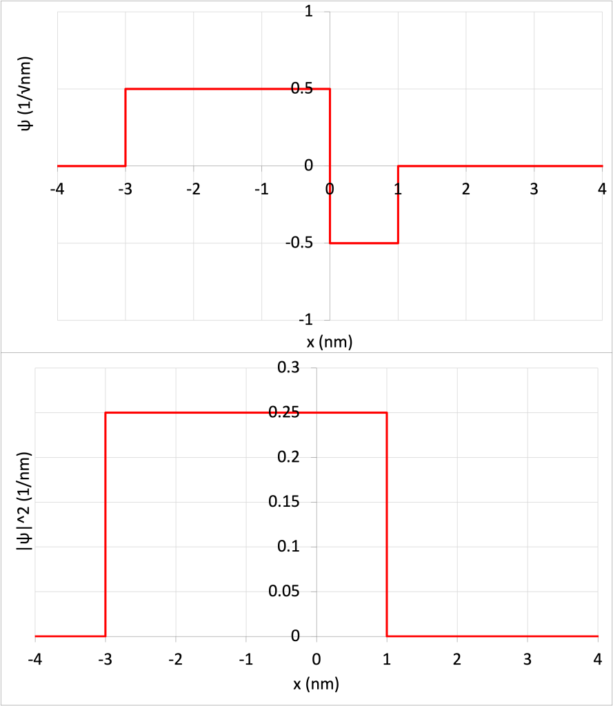
The particle can only exist in the range of -3 nm and 1 nm. In other words, there is 0% probability that the particle will exist at a value of x less than -3 nm or greater than +1 nm.
The odds that the particle will be found between the range of -3 nm and +1 nm should be 100%. This can be confirmed by calculating the area of the wave function squared in this range, illustrated as a shaded area in Figure 32.4.
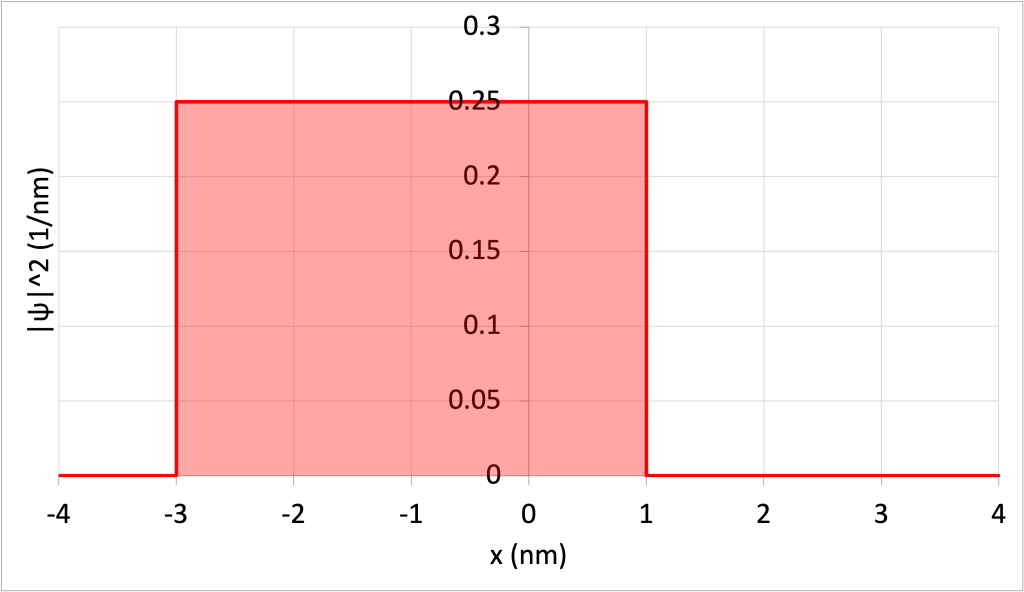
The area of the rectangle is equal to the probability, which is equal to

The probability of finding the particle within the range of -3 nm and 0 nm (illustrated as a shaded area in Figure 32.5.
The area of this rectangle is equal to

As far as atoms go, Schrödinger’s equation has only been solved exactly for the hydrogen atom, which consists of one proton and one electron. It can also be solved exactly for individual particles such as a single proton, or electron, in a few simple environments. When using Schrödinger’s equation to model complicated particles or atoms that have more subatomic particles than hydrogen, computers need to be used to numerically calculate wave functions.
The major limitation of Schrödinger’s equation is that it is very complicated to use, to the point where solving it analytically (in essence, solving an equation “by hand” by using mathematical operations) quickly becomes impossible. Also, the wave function only tells us probabilistic information about quantum particles. The quantum universe is indeed much different from the classical universe!
The observer effect
The observer effect occurs when measuring a quantum process. When making an observation, we influence that process in some way and therefore affect the outcome. This doesn’t only happen in quantum systems, it also happens in classical systems. To measure the tire pressure in a car or bicycle tire, some of the air in the tire is let out when connecting the tire pressure gauge. This changes the measurement. Whatever pressure is measured is going to be slightly less than the pressure that existed in the tire before it was measured. Another example is measuring the temperature of a substance with a thermometer. As the substance and thermometer reach equilibrium, some energy must transfer between the two. This changes what the temperature of the substance was (even if only slightly) before the thermometer was introduced.
Most of the time, our influence on the outcome of a classical or macro-scale measurement is negligible. When using an ultrasonic sensor to measure the speed of a cart in a physics experiment, a sound wave is bounced off of the cart. There is going to be energy and momentum transfer between the sound wave and the cart, but the speed and momentum of the cart will not change to any noticeable degree as a result of using sound waves to measure them. We can essentially ignore the observer effect in cases such as this.
In particle physics, measuring the speed of an electron requires hitting it with a photon. Unlike the sound wave and the cart, an electron is a subatomic particle that will experience non-negligible changes when it interacts with a photon. When measuring the electron by hitting it with a photon, the electron can be affected to a significant degree.
There is a quote in the book Perpetual Motion by Alec Thompson Stewart that does a great job summing this up:
“Perhaps the most gentle method of searching for an electron in an atom in order to measure its speed is to shoot another electron through the atom. If the exploring electron hits an electron in the atom, it is deflected and from the angle it may be possible to obtain the velocity of the electron it hit. From the atom’s point of view, this technique is not exactly subtle. It would be like closing one’s eyes and driving full speed through a street intersection to find out whether traffic was moving on the cross street. If a collision occurred, one could assume that there was a car on the cross street.”
When we measure a quantum object, we affect its outcome and cause the wave function to take on one particular value. This is known as collapsing the wave function. Whereas prior to our measurement an electron could have had one of many different values for momentum (for example), after measurement, we know exactly what that value is. The wave function has collapsed.
Relevant to this topic is a thought experiment known as Schrödinger’s cat. First, it is important to point out that this is a thought experiment, and was not actually performed, nor were any cats harmed. It only serves as a metaphor to illustrate some of the bizarre interpretations of quantum mechanics. The thought experiment takes a cat, a flask of poison, a Geiger counter, and a radioactive source in a box. The radioactive source has a 50% chance of decaying and emitting a particle within a certain time frame that can be measured by a Geiger counter. If the decay particle is measured by the Geiger counter within the time frame, the flask of poison is shattered and the poison is released, killing the cat. If the detector does not record the particle within the time frame, the mechanism is prevented from shattering the flask. This is depicted in Figure 32.6.
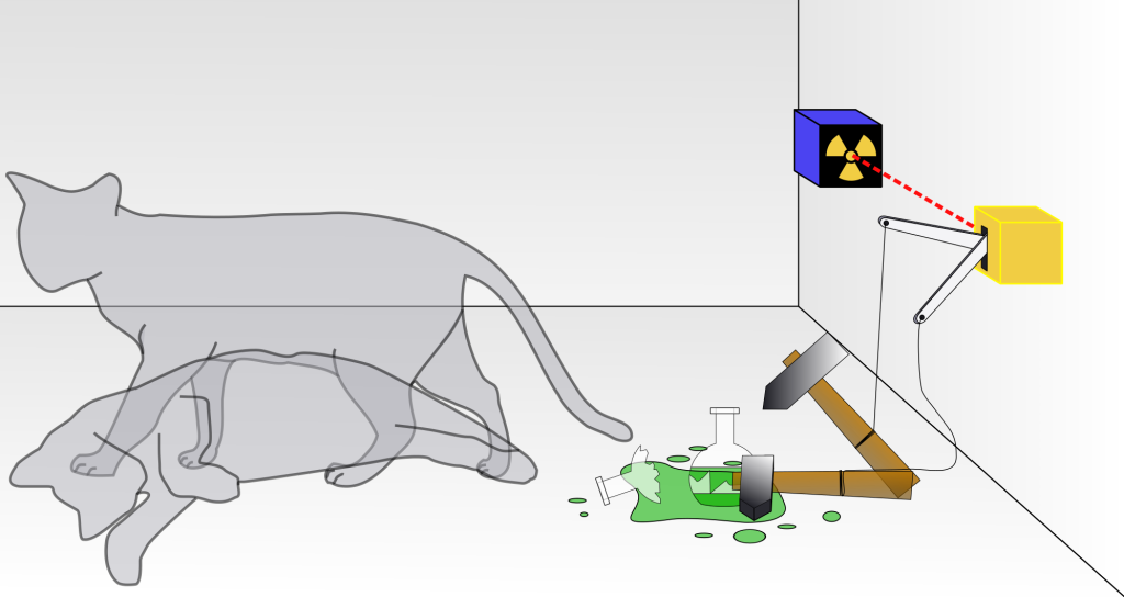
The question is: after the allowed time interval, is the cat alive or is the cat dead? This determination cannot be made without opening the box and taking a look. One interpretation of quantum physics states that, after the time frame, the cat is both alive and dead. It exists in a so-called superposition of both states. It is not until the box is opened that we observe the cat to be in one or the other state, collapsing the wave function of the cat into either the “alive” state or the “dead” state with 50% probability of either state being the outcome.
There are a lot of arguments and interpretations of this thought experiment, and it has led to rigorous debate between physicists.
Quantum tunneling
Consider throwing a bouncy ball at a wall. Assuming you don’t throw the ball so fast that it smashes through the wall, it will predictably bounce back to you. This is a classical particle: a large object that obeys the laws of classical physics. Its wave nature is so trivial that it can be completely ignored.
If instead you throw an electron at a barrier, it is possible that the electron will tunnel through. During that process, the barrier won’t be damaged or changed, but the electron will simply pass through it. This is due to the wave-like nature of quantum objects. This phenomenon is known as quantum tunneling.
The simulation in the video below shows the wave function of a quantum object as it travels toward a barrier. While most of the object reflects off of the barrier, a small amount tunnels through.
If you think this sounds bizarre, consider that the solid-state memory used in your USB drives, smartphone, and possibly computer or laptop, uses quantum tunneling to store data in its flash memory. Electrons tunnel through an insulating barrier and get stored to save your files, text messages, and photos as binary data. This is a real phenomenon that only occurs with regularity on the quantum level.
Quantum entanglement
Quantum entanglement describes the process during which two or more quantum objects interact in such a way that their quantum properties become interrelated. For example, two photons can be generated such that one has a vertical polarization and the other has a horizontal polarization. The two photons have mutually perpendicular polarizations. This means that if you were to measure the polarization of one of the photons, you would instantly know the polarization of the other, as the two are perpendicular to each other.
The aspect of quantum entanglement that is particularly fascinating has to do with the implications of having simultaneous knowledge of both particles. Imagine that a physicist named Alice entangles two photons in polarization. Alice keeps one photon traveling in an optical setup nearby, and sends the other one to a friend (Bob) on another planet, or even on the other side of the Earth. If Alice measures the polarization of her photon, she instantly knows the polarization of the other photon. Scientists were initially concerned that this seems to imply that knowledge moves faster than the speed of light. If the second photon is on Jupiter, Alice knows its polarization without having to travel all the way there to measure it!
The fact is, however, that by the time Alice calls Bob to tell them the results of the polarization measurement, the transmission of that information to Bob will obey the universal speed limit. Bob will not know the outcome faster than light speed, as Alice’s message must travel at or below the speed of light to reach them. While Alice may know information about both particles, that information cannot be transmitted faster than the speed of light.
This is an active area of research for use in quantum computing. Due to the amount of information that can be encoded into entangled quantum particles, the hope is that quantum computing can solve problems that would take classical computers an enormous amount of time to solve.
Further reading
- The Schrödinger equation explained – This short video describes the Schrödinger equation.
- Rigden, J. S. (2002). Hydrogen: The Essential Element. Harvard University Press
- What is quantum entanglement? – This article from Astronomy magazine explains the concept of entanglement.
- Einstein’s ‘spooky action at a distance’ spotted in objects almost big enough to see – This article from Science magazine discusses the entanglement of particles that are almost on the macro scale.
Practice questions
Numerical analysis
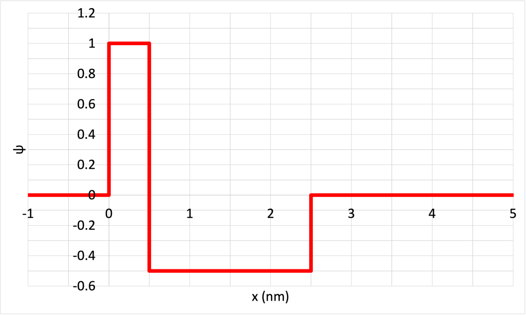
- Consider the contrived wave function for a hypothetical particle shown in Figure 32.7. (Download this data [XLSX, 9 kB]) Determine the probability of finding the particle in the following ranges:
- 0 < x < 0.5 nm
- 0.5 nm < x < 2.5 nm
- 1 nm < x < 2 nm
- x < 0
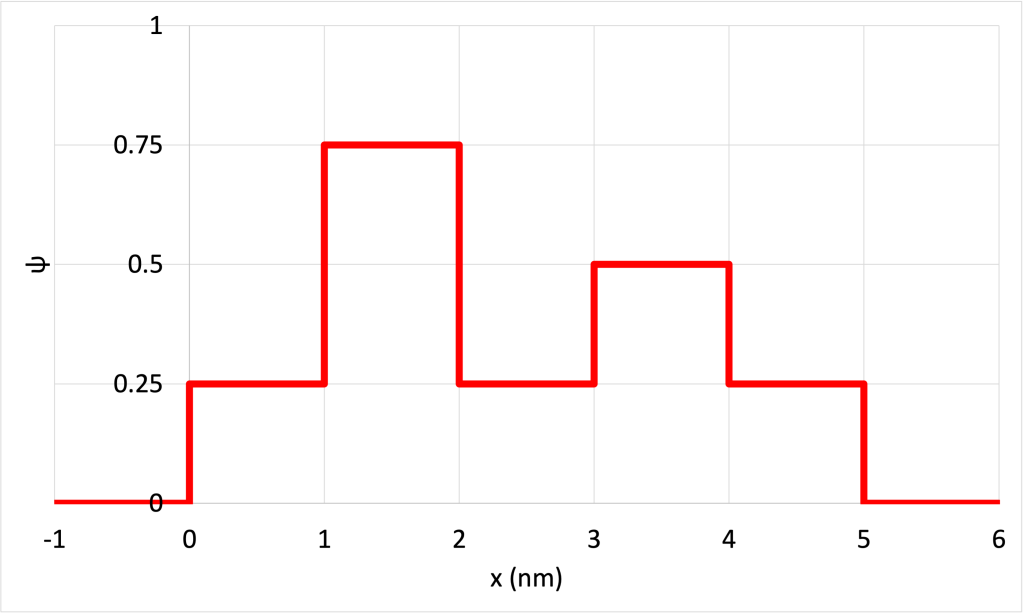
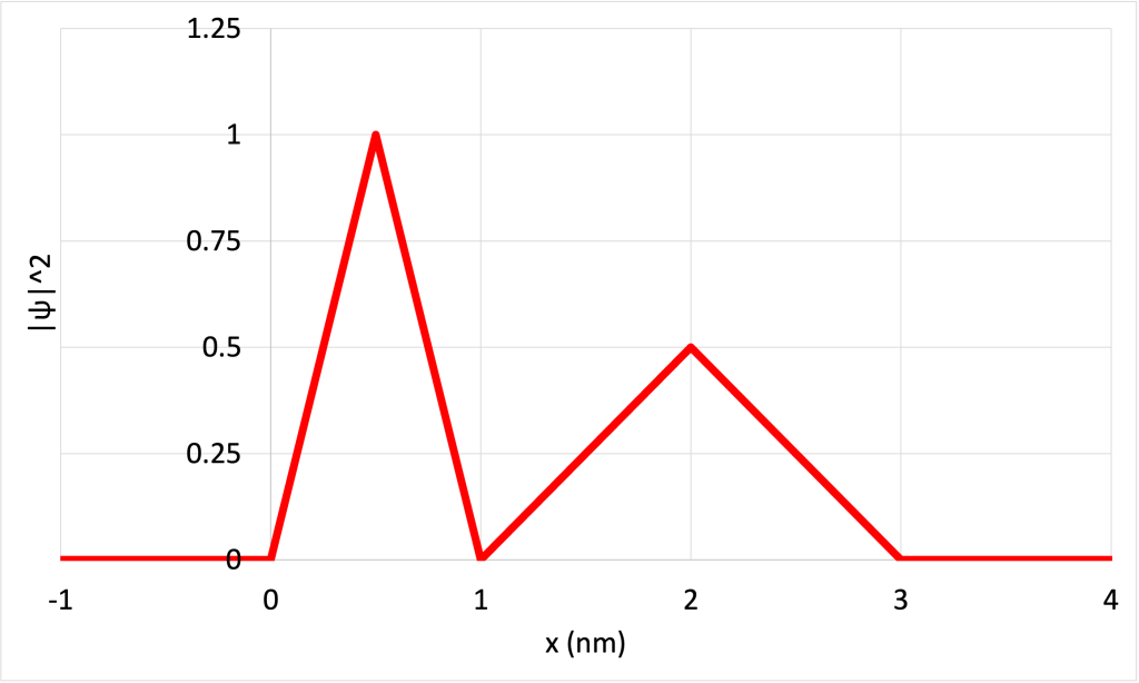
- Consider the contrived wave function for a hypothetical particle shown in Figure 32.8. (Download this data [XLSX, 9 kB]) Determine the probability of finding the particle in the following ranges:
- 0 < x < 1 nm
- 1 nm < x < 2 nm
- 3 nm < x < 4 nm
- 1.5 nm < x < 3.5 nm
- 0 < x < 5 nm
- Figure 32.9 shows a contrived plot of for a hypothetical particle. (Download this data [XLSX, 9 kB]) Determine the probability of finding the particle in the following ranges:
- 0 < x < 1 nm
- 1 nm < x < 2 nm
- 0.5 nm < x < 2 nm
- 1.5 nm < x < 3 nm
- x > 3 nm
The collection of frequencies of light emitted by a substance via the electron deexcitation process is known as its emission spectrum. It appears as bright lines on a dark background.
An element is a substance that consists of atoms whose nuclei have the same atomic number. An element cannot be broken down further by chemical means.
Electron deexcitation is the process by which an electron loses energy and jumps down one or more energy levels. In the process, the electron either transfers energy to another particle, emits a photon, or generates heat.
Gas is a state of matter where molecules are very free to move about and generally do not interact with each other except during collisions. This means that the shape and volume of a gas is free to change. Gas is one of the four most common phases of matter.
Electron excitation is the process by which an electron gains energy and moves up one or more energy levels.
An absorption spectrum shows the wavelengths of light that are absorbed by a material. It appears as a continuous spectrum with dark lines caused by light passing through a substance.
The wavelength of a wave describes the shortest distance between two identical repeating points on a wave. (symbol: λ, unit: m)
The electromagnetic spectrum describes the entire range of electromagnetic waves. Each subset of waves can be defined in different categories based on its frequency or wavelength.
Classical physics describes the natural phenomena that can be explained by Newton’s laws of motion, Maxwell’s equations, and the laws of thermodynamics.
An electron is a fundamental building block of matter that has a negative charge and is found surrounding the nucleus of an atom.
The orbit of an electron describes the properties of the electron wave as it exists around the nucleus of an atom.
A proton is a subatomic particle that has a positive charge and resides in the nucleus of an atom.
The orbit of a satellite describes its path around a planet or star.
Gravity is the attractive force experienced by objects of mass. It is one of the four fundamental forces.
Energy levels describe the quantity of energy that each electron orbiting an atom can have. Each atom is uniquely defined by its discrete energy level values. The lowest energy level is known as the ground state.
Path describes the total distance that an object travels as it moves from one point to another, measured along its trajectory. It is a scalar quantity. (symbols: d, x [for horizontal path], y [for vertical path], unit: m)
Electromagnetism describes the interactions that occur between charged objects.
Energy is defined as the capability of an object (or collection of objects) to do useful work. (symbol: E, unit: J)
A wave is a periodic oscillation that transfers energy from one place to another.
A standing wave is a wave that oscillates in time but that does not move in space. Standing waves occur due to interference between two waves that have equal amplitude and frequency that travel in opposite directions.
Interference is the phenomenon that occurs when two waves overlap. The total amount of wave energy present at a point is equal to the sum of each individual wave's energy at that point.
Momentum is a vector property that quantifies the motion of an object. It is sometimes called "inertia in motion" as it is the product of mass and velocity. (symbol: p, unit: kgm/s or Ns)
The uncertainty principle theorizes the extent to how well we can know information about related properties.
Electric charge is a fundamental property of matter that causes particles that carry a charge to experience a force when in the presence of an electric field.
Current describes the flow of electric charge through a circuit. (symbol: I, unit: A)
A hypothesis is a proposed explanation of how the universe works that is based on observations and can be tested experimentally.
Physics is a branch of science that focuses on the fundamentals of the workings of our universe.
Kinetic energy is the energy that an object has due to its motion. (symbol: KE, unit: J)
Potential energy is energy that exists based on the arrangement or configuration of a substance.
Mass is a property of physical objects that relates to resistance to changes in motion: inertia. (symbol: m, unit: kg)
The observer effect describes the process that occurs when measuring a quantum process. When making an observation, the process is influenced in some way, and therefore affects the outcome.
Pressure defines the amount of force applied over an area of a substance. (symbol: P, unit: Pa)
Temperature defines the average kinetic energy of an object. It quantifies the “hotness” or “coldness” of something. (symbol: T, unit: °C or K)
Ultrasound is the set of sound waves that have frequencies above 20,000 Hz. They are not audible to humans.
Speed is the scalar quantity that describes the rate at which an object changes its position. Speed is equal to position divided by time. (symbols: s, |v|, unit: m/s)
A sound wave is a longitudinal wave that is caused by vibrations in air pressure between two points.
Quantum physics describes the physical laws used to describe the properties of matter and energy that occur on a very small scale.
A scientific law is a statement that describes relationships among the quantities that we observe or measure.
Polarization is the property of transverse waves which allows them to have their electric field components oscillating in a single direction.
