25. Electromagnetic induction

Faraday’s law

Recall from the previous chapter of this book that it is possible to create magnetism from electricity. Moving charges can create a magnetic field. This is how electromagnets work.

As it turns out, it’s also possible to generate electricity from magnetism. In the video below, Dr. Pasquale has connected a coil of wire to a galvanometer, which measures electric current. As she moves a magnet into the coil of wire, the galvanometer indicates that current is flowing through the circuit.

Whenever there is a moving magnetic field in the vicinity of an electric circuit, that changing magnetic field will induce a voltage. When there is a closed circuit, that voltage will create a current, as described by Ohm’s law.

Faraday’s law of induction can be used to quantify the strength of this induced voltage. Faraday’s law is a complicated equation (requiring calculus), so we will not use the exact equation in this textbook. Instead, we will learn the qualitative properties of Faraday’s law.

Faraday’s law states that the strength of the induced voltage is proportional to the strength and rate of change of the magnetic field, the number of coils in the wire, and the cross-sectional area of the coil of wire.

The stronger the magnetic field of the magnet being used, the larger the induced voltage will be. This effect is demonstrated in the video below where Dr. Pasquale uses small and large magnets to generate induced voltage. The two magnets are otherwise identical except for their size (they have the same area and are made of the same magnetic material), so in this case, the size of the magnet is a good proxy for strength. The galvanometer deflects much less (as there is much less current flow as a result of the smaller induced voltage) for the small as compared to large magnet. Dr. Pasquale did her best to control all other variables (the coil is the same for both trials, and she did her best to move both magnets at the same speed).

The faster the motion of the magnetic field (with respect to the coil of wire), the larger the induced voltage. This relative motion between the magnet and the coil creates a rate of change of the magnetic field. An increasing amount of magnetic field penetrates the coil when the magnet and coil move toward each other and a decreasing amount of magnetic field penetrates the coil when the magnet and coil move away from each other. This is demonstrated in the video below. When Dr. Pasquale moves the magnet into the coil slowly, the galvanometer registers a small amount of current. When she moves the magnet faster, the galvanometer registers a larger amount of current. Note that if the magnetic field does not move, there will be no induced voltage, and therefore no current.

Faraday’s law tells us that the magnetic field must be changing within the coil of wire to induce any voltage. If the magnet is held stationary, then the coil of wire can be moved to create this relative motion.

The induced voltage is also proportional to the number of turns and cross-sectional area of the coil of wire. A coil with one or two turns will not experience as much induced voltage as a coil with hundreds or thousands of turns. A coil with a small diameter will have less induced voltage than a coil with a large diameter.

In the video below, this property is demonstrated. As Dr. Pasquale does not have two coils of wire with identical cross-sectional areas and only differing number of turns, or with the same number of turns and different cross-sectional areas, it was not possible to control for either of those two variables. However, she does have a coil of wire with a small area and fewer turns than another coil, which has a large area and much more turns. As Dr. Pasquale moves the magnet, attempting to keep the speed as constant as possible, through both coils, the current measured by the galvanometer is greater in the larger coil with more turns.

The sign of the induced voltage has to do with three things: which pole of the magnet is used, if the magnet is entering or leaving the coil, and which side of the coil (left or right) it is moving toward or away from. By reversing any one of these three things, the sign of the induced voltage will become the opposite of what it was previously.

In the videos below, Dr. Pasquale creates several different scenarios of moving a magnet into and out of a coil of wire (using different poles, entering and leaving the coil, and entering/leaving from different sides of the coil). As a baseline, Dr. Pasquale inserts the north pole of the magnet into the right side of the coil. This causes the galvanometer to deflect left, which indicates a negative voltage and current.

When Dr. Pasquale then removes the north pole of the magnet from the right side of the coil, the sign changes and the galvanometer deflects right, indicating a positive voltage and current. (One of the three conditions – insertion / removal – was changed from the baseline condition, causing the sign to switch once from negative to positive.)

Dr. Pasquale then changes the magnetic pole and inserts the south pole of the magnet into the right side of the coil. This causes the galvanometer to deflect right, which indicates a positive voltage and current. (Because one condition was changed from the baseline, the sign switches once from negative to positive.)

Then, Dr. Pasquale switches sides of the coil and inserts the north pole of the magnet into the left side of the coil. This causes the galvanometer to deflect right, which indicates a positive voltage and current. (Again, because one condition was changed from the baseline, the sign switches once from negative to positive.)

Note that changing two of these variables simultaneously will cause an effect that cancels itself out (this is similar to multiplying a value by negative one twice, the minus sign cancels out). This is demonstrated at the end of the above video when Dr. Pasquale removes the north pole of the magnet from the left side of the coil. This causes the galvanometer to once again deflect to the left, indicating a negative voltage and current. Changing three of these variables simultaneously will cause the current to change its sign from the baseline scenario.

Lenz’s law

When a conductor moves through a magnetic field (or when a magnetic field moves around a conductor), that changing magnetic field creates an induced voltage. A voltage in a conductor will give rise to electric current. In this case, that current is known as an eddy current. Lenz’s law defines the direction that eddy currents will be generated. It states that the current induced in a conductor will itself generate a magnetic field that opposes the magnetic field that induced the current.

This effect can be demonstrated by dropping a magnet down a copper pipe. The falling magnet is a moving magnetic field, and the copper pipe is a conductor. The eddy currents generated in the copper pipe will oppose the magnetic field that created them. This causes a repulsion effect between the two magnetic fields, causing the magnet to move much slower than we would expect due to the acceleration due to gravity. This is demonstrated in the video below. First, a small piece of nonmagnetic metal is dropped down the copper pipe to demonstrate the motion of an object acting only under the influence of gravity. Then, a small magnet is dropped down the copper pipe. Its motion is much slower than that of the nonmagnetic object.

This effect of slowing motion has practical effects. Induction braking (also known as eddy current braking) uses the drag between an external magnet and eddy currents generated in a moving or rotating conductor to slow something down. Induction braking is used in vehicles such as high-speed trains. Because no parts directly touch during the induction braking process (as would occur during friction braking, where a brake pad creates a friction force to slow down a moving object), induction braking leads to less wear on parts.

The video below demonstrates this induction braking process. A pendulum consisting of an aluminum (conducting) plate is capable of moving back and forth with regular periodic motion. Once a magnet is placed in the path of the pendulum, the currents induced in the conducting plate are directed to oppose the changing magnetic field intercepting the plate. The induction braking process occurs as the eddy currents induced in the plate experience a magnetic force that slows the pendulum and brings it to an abrupt stop.

Generators and motors

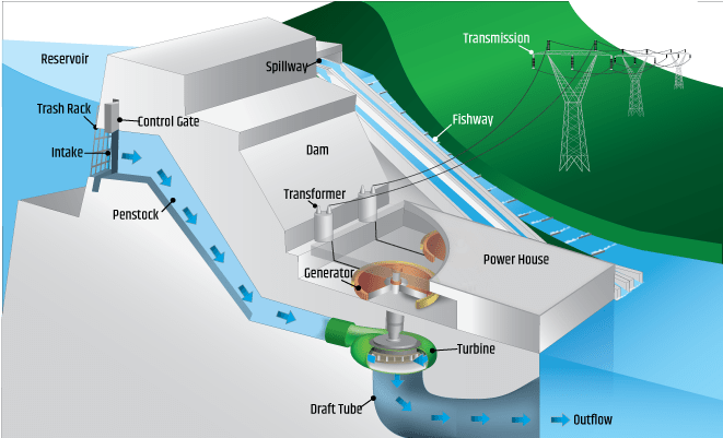
The induction of electric potential (as discussed earlier in this textbook, voltage is a difference in electric potential between two points) in a circuit allows us to create generators. Coal, gas, and nuclear power plants work by heating water into steam. That steam spins a turbine that either moves a magnet around a coil of wire, or moves a coil of wire around a magnet. Wind turbines create this relative movement of a magnet and coil of wire using the power of moving air causing the blades of the generator to rotate. Hydroelectric power plants harness the power of falling water to create this motion. A schematic of a hydroelectric power plant is shown in Figure 25.1.

In the video below, Dr. Pasquale created a generator out of a salad spinner and two coils of wire. Permanent magnets have been placed at regular intervals around the perimeter. When Dr. Pasquale rotates the salad spinner, the magnetic fields rotate. That rotation causes motion, and when the magnets move past the coils of wire, voltage is generated.

When Dr. Pasquale connects the output of the generator to a multimeter, we can see the effect of the generator on the average current that is produced. The slower she spins the generator, the smaller the voltage and current that’s generated. The faster she spins the generator, the larger the voltage and current that’s generated. That makes sense based on Faraday’s law of induction.

The voltage created by a generator is AC. As we saw when looking at how the sign of the induced voltage changes in Faraday’s law, having a pole move toward or away from a coil of wire will cause a difference in sign. In that particular example, when the north pole moved toward the coil, the sign was positive. When the north pole moved away from that same coil, the sign was negative. In the case of the salad spinner, north and south poles are constantly rotating toward and away from the coils of wire, causing the sign of the induced voltage (and current) to periodically change sign. This is alternating current. This is shown for the salad spinner in the video below where Dr. Pasquale connected the output of the generator to an oscilloscope. (Note that the signal on the oscilloscope is AC but not sinusoidal. This is possibly due to the magnets each having a slightly different strength or not being equally spaced and therefore not generating a “clean” signal.)

In summary, a generator is a device that converts mechanical work to electrical energy. The opposite process is also useful. A device that converts electrical energy to mechanical work is known as a motor. (We saw an example of a DC motor in the previous chapter in this textbook.)

The video below demonstrates the fact that a generator and motor are the same concept working in reverse. Dr. Fazzini and Professor Nikolova both hold handheld generators/motors. First, Professor Nikolova uses her handheld device as a generator (using mechanical work to generate electrical energy), which sends electrical energy to Dr. Fazzini’s device, causing it to rotate as a motor would (using that electrical energy to generate mechanical work). Then the process occurs in reverse. Dr. Fazzini uses his device as a generator, which causes Professor Nikolova’s device to act as a motor.

Transformers

A transformer is an electronic device that is capable of transferring energy from one circuit (known as a primary circuit) to another (known as a secondary circuit) with no physical connection existing between the two circuits. A transformer can also change the value of the voltage induced in the secondary circuit compared to the voltage in the primary circuit, either increasing it or decreasing it. This device brings together what we’ve learned in this and the previous chapter in this textbook: electric current flowing through a coil of wire generates a magnetic field. When that current is AC, the electric field changes, which generates a changing magnetic field. That changing magnetic field causes an induced voltage in any coils of wire that are nearby.

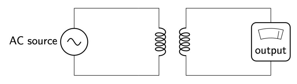
The symbol for a transformer used in a circuit diagram looks like two coiled objects that are near each other. The circuit diagram in Figure 25.2 depicts a primary coil (on the left) powered by an AC voltage source connected to one coil of a transformer. The secondary coil (on the right) is connected to a galvanometer which can show the output voltage induced in the secondary by the primary.

In the video below, Dr. Pasquale has two coils of wire located near each other. One of the coils, called the primary, is connected to an AC voltage source (this is the large rectangular box located in the bottom right of the video). This generates a changing magnetic field in the primary coil. That changing magnetic field is large enough to overlap with the secondary coil, inducing voltage in the secondary coil. We can see that on the galvanometer connected to the secondary. Because the secondary is connected in a complete circuit, current flows. This current is also AC.

While the primary and secondary coils are not physically connected, the effectiveness of the transformer is limited by how far away the two coils are positioned. This is shown in the video below. As Dr. Pasquale separates the two coils of wire, the induced voltage decreases, demonstrated by the swings on the galvanometer becoming smaller in magnitude.

At a certain point, if the secondary coil moves too far from the primary, the changing magnetic field no longer overlaps with the secondary, and no voltage is induced. This is not a long-distance phenomenon.

It’s possible to increase the effectiveness of this process by placing an iron core into the two coils of wire. This increases the strength of the induced voltage because the magnetic domains in the iron core will be aligned by the magnetic field generated in the primary. That will cause a further boost to the strength of the magnetic field by increasing how well the primary and secondary devices are coupled together. This is demonstrated in the video below. When Dr. Pasquale places an iron core into both coils of wire, the swings on the galvanometer become much larger, demonstrating a much larger induced voltage.

In the video below, Dr. Pasquale connects the primary to a direct current (DC) source, a battery. In this case, the galvanometer on the secondary no longer deflects. After Dr. Pasquale closes the switch, the primary coil is connected to the source, as indicated by the glowing light-emitting diode inserted into the primary circuit to demonstrate that it is complete. Therefore, the primary circuit is generating a magnetic field. However, that magnetic field does not change over time. It is static. Faraday’s law of induction tells us that the only way to generate electricity is to have a changing magnetic field. That requirement is not satisfied in this circuit. Therefore, no voltage is induced in the secondary and no current flows in the secondary.

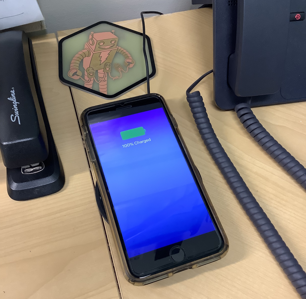
Wireless induction can be extremely useful, and today we benefit from technology that uses short-range induction to wirelessly charge our smartphones and other devices. Dr. Pasquale’s phone is seen wirelessly charging in Figure 25.3.

Transformers aren’t just useful for letting us charge smartphones and other devices. They are also an essential circuit component used to change the value of voltage between circuits. It is possible to create a step-up transformer that creates more voltage on the secondary than the primary. It is also possible to create a step-down transformer that creates less voltage on the secondary than the primary.

Whether or not a transformer is a step-up or step-down (or if it does not change the voltage at all) has to do with the number of turns of wire in each transformer. For an ideal transformer (one with no losses and experiencing perfect coupling between both coils of wire), in equation form, this can be written as

The voltage on the primary () divided by the number of turns in the primary coil () equals the voltage induced in the secondary () divided by the number of turns in the secondary coil ().

If, for example, a primary coil has 6000 turns and is powered by a 120 V AC source. If the secondary coil has 2000 turns, we can calculate the induced voltage on the secondary coil.

This is a step-down transformer, because the voltage on the secondary is less than the voltage on the primary.

If, instead, a primary coil has 500 turns and is powered by a 5 V AC source, and the secondary coil has 5000 turns, we can calculate the induced voltage in the secondary.

This is a step-up transformer, because the voltage on the secondary is greater than the voltage on the primary.

A step-up transformer sounds pretty great: it generates more voltage in the secondary than existed in the primary! At this point, you’re probably very familiar with conservation laws (particularly, that energy cannot be created or destroyed). The voltage induced in the secondary coil does not come for free. We can use the power equation () to determine what property is therefore affected in the secondary. Power (being the rate of energy consumption in a circuit element) will be equal in both the primary and the secondary under ideal conditions. In other words,

The product of voltage and current in the primary must be equal to the product of voltage and current in the secondary.

A helpful analogy may be to consider a transformer to be the electrical version of a mechanical lever. As previously discussed, a lever allows us to trade force for distance (and vice versa), allowing us to move a heavy output weight with a small input force, at the cost of moving a longer distance on the input than is achieved on the output. A transformer allows us to trade voltage for current (and vice versa).

If the primary device has a 5 V AC source, and contains 10 of resistance, then we can use Ohm’s law to calculate the current in the primary to be 0.5 A. The power consumed by the primary is 5 V times 0.5 A: 2.5 W. The power consumed by the secondary must be 2.5 W as well. If the voltage generated on the secondary is 50 V, we can calculate that the current flowing through the secondary will be limited to 0.05 A, or 50 mA.

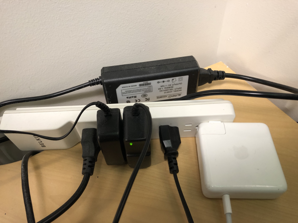
Cables used to charge household electronics are frequently connected to a transformer. The voltage we have access to in homes in the United States is 120 volts AC. Most modern electrical devices require DC voltage at a much lower value, usually between 5 and 12 volts.

The large blocky part of our charging cables, colloquially referred to as a “wall wart” (four examples of which are shown in Figure 25.4), contains a step-down transformer to convert the 120 volts to a smaller value. Then, a rectifier is used to convert that AC voltage to a DC voltage, using a process we discussed in a previous chapter of this textbook. Finally, there is usually some noise-reducing circuitry inside that “wall wart” to ensure that no voltage spikes get through to harm our electronic devices.

While we’ve discussed the transmission process in terms of voltages and coils of wire, in fact, it is the presence of changing electric fields that causes changing magnetic fields, and changing magnetic fields that cause changing electric fields. This induction process does not require the presence of any circuitry to occur. In fact, electromagnetic fields are all around us!

Power distribution and transmission

Now that we’ve learned about how power plants generate electricity, we can discuss how that electricity gets distributed to businesses, schools, and homes. The overview of this process is shown in Figure 25.5, which highlights the generation, transmission, and distribution process.

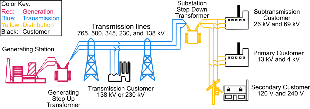
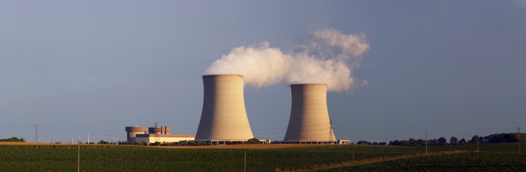
The process starts at a power plant, most of which generate power using a turbine. Depending on the type of power plant: nuclear, coal, gas, or wind, the power generated by a power plant will be vastly different. As an example, the Byron Nuclear Generating Station in Ogle County, Illinois (shown in Figure 25.6), has a capacity of approximately two gigawatts. That is: two billion watts of power.

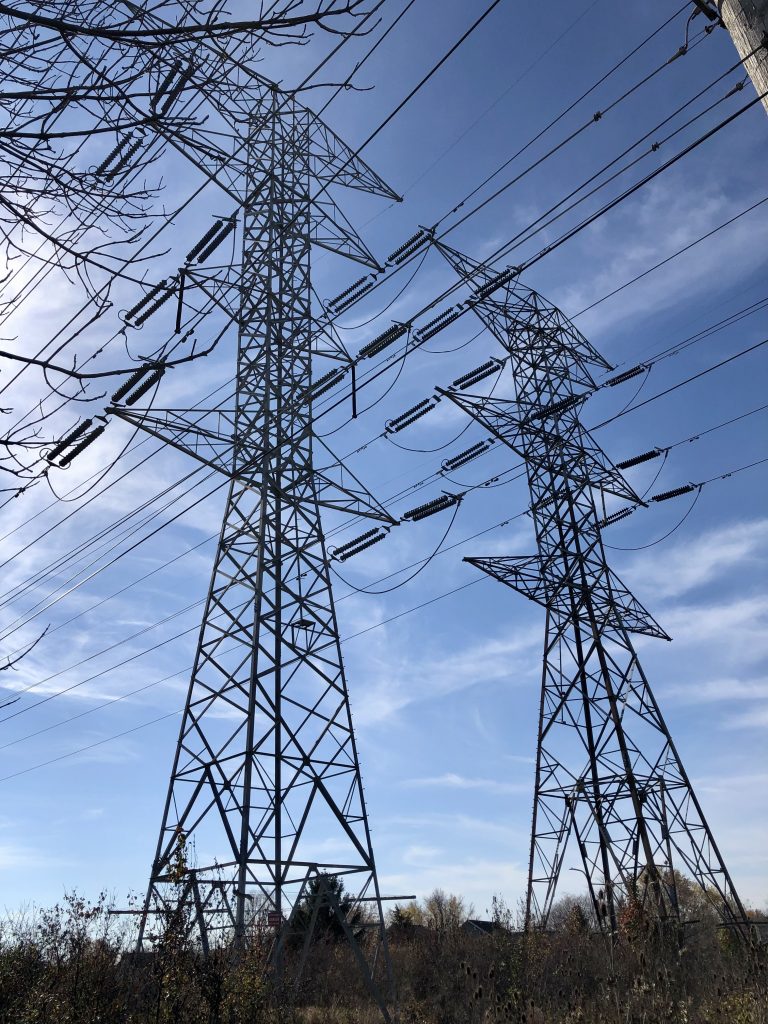
The voltage of the electricity generated by a power plant is typically about 25,000 V (25 kV). The frequency of the AC voltage is 60 Hz in the United States. This voltage is stepped up at the power station to a much larger voltage before being sent through transmission lines on the next phase of its journey. These are the extremely huge and tall power lines that do not route electricity to buildings, but instead transmit electricity over long distances. A photograph of transmission lines in Elgin, Illinois, is shown in Figure 25.7.

The voltage through transmission lines varies, but is usually in the neighborhood of 200 kV to 500 kV. Why is such high voltage used in transmission? Remember that power is conserved in the transmission and distribution process. Using the Byron power plant as an example, if two billion watts of power is generated, and that power is sent through transmission lines at 25,000 V (source [PDF, 18 kB]), then the current will be 80,000 A. The voltage is stepped up at the power plant and sent through the transmission system at 345,000 V. Because power is conserved, the current in the transmission lines will ideally be approximately 5,800 A. In this example, the voltage is stepped up by a factor of 13.8. This requires that the current is decreased by the same factor. Due to the resistance of the transmission lines, the current causes heating and energy losses in the transmission process. The rate of the thermal losses is . So, the higher the voltage, the smaller the current, and the more efficient the transmission process will be. In this example, the current being reduced by a factor of 13.8 reduced the power losses by a factor of 190.

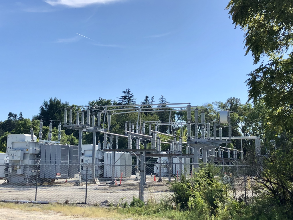
At the end of transmission lines is an electrical substation. At this point, the voltage from the transmission lines is stepped down again. The exact voltage level varies depending on the customer(s) ultimately receiving the power. Distribution to neighborhoods will typically be less than 34,000 V (source [PDF, 327 kB]). This power is sent through distribution lines. A suburban substation in DuPage County, Illinois, is shown in Figure 25.8.

Distribution lines are much smaller than transmission lines and send power from the substation to neighborhoods. These are the power lines you will typically see on the sides of the road in the United States (shown in Figure 25.9). Sometimes they are underground, which prevents power outages from heavy winds, fallen tree branches, and winter storms. Because distribution lines are located in neighborhoods, and only transmit electricity over short distances, for safety reasons, the voltage can and should be much lower than what is used in long-distance transmission lines.

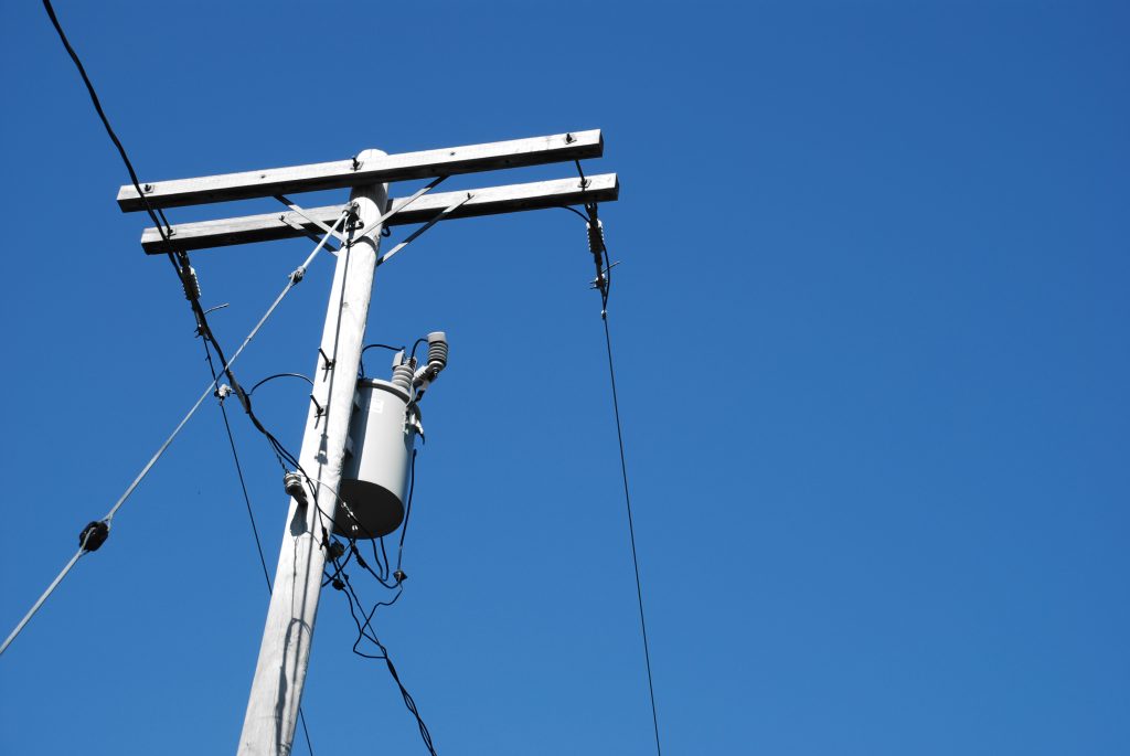
Transformers on the power poles holding up distribution lines (the cylindrical shaped object in Figure 25.10 contains a transformer) steps down the voltage once more to 240 V for use in residential homes. Some large consumer appliances such as clothes dryers may require this high voltage level. This voltage is then divided into 120 V which is sent to most of the outlets in a household.

While the voltage of the electricity is changed throughout this journey from the power plant, the frequency of the AC voltage remains 60 Hz the entire time, which is why we obtain 60 Hz electricity from wall outlets in the United States.

Further reading

• Power grid? What is that? [PDF, 251 kB] – This article from IEEE Potentials magazine talks about the development of the power grid in the United States.
• How it works [PDF, 34 kB] – This informative article from the US Department of Energy has a lot of information about the power transmission and distribution process in the United States.
• The Power Grid – This interactive website lets you determine the effect of power consumption and generation on the power grid.
• Overhead transmission lines – This illustrated glossary of transmission lines from OSHA shows how the voltage of transmission lines can be determined from the design of the towers.
• Electricity 101 – This list of FAQs from the US Department of Energy answers a lot of common questions about power generation, transmission, and distribution in the United States.
• How Solar Storms Could Knock Down Our Power Grid – This video from PBS explains how the electrical grid (particularly in North America) can be susceptible to interruptions from strong solar activity.

Practice questions

Conceptual comprehension

1. A primary coil contains 50 turns and is connected to a secondary coil that contains 100 turns. Is this a step-up or step-down transformer? How do you know?
2. A primary coil contains 50 turns and is connected to a secondary coil that contains 10 turns. Is this a step-up or step-down transformer? How do you know?

Numerical analysis

1. A step-up transformer has 400 turns in the primary coil and increases the voltage from 110 V on the primary to 550 V on the secondary. Calculate the number of turns in the secondary coil.
2. The primary voltage of a step-up transformer is 240 V, with a secondary voltage of 4800 V. If the primary has 200 turns, calculate the number of turns in the secondary coil.
3. The primary voltage in a step-up transformer is 120 V, which generates a secondary voltage of 600 V. If the secondary coil contains 150 turns, calculate the number of turns in the primary coil.
4. The primary voltage of a step-down transformer is 480 V, which induces a secondary voltage of 120 V. If the primary contains 400 turns, calculate the number of turns in the secondary coil.
5. A step-down transformer decreases the voltage from 150 V to 30 V. The secondary contains 50 turns. Calculate the number of turns on the primary coil.
6. For a step-up transformer with a primary voltage of 200 V, a secondary voltage of 1000 V, and a current of 4 A in the secondary, calculate the power consumed by both the primary and secondary coils.
7. A step-up transformer has a primary voltage of 120 V and a secondary voltage of 600 V. If the current in the primary coil is 5 A, calculate the current flow through the secondary circuit.
8. In a step-down transformer, the primary voltage is 240 V, and the secondary voltage is 120 V. If the current in the secondary coil is 2 A, calculate the current flowing through the primary circuit.